Yueheng Zeng @ Project 2
This project explores various techniques in image processing, focusing on 2D convolutions and frequency-based transformations. The goal is to build foundational intuitions about how filters affect images and to experiment with advanced image manipulation techniques, including sharpening, hybrid image creation, and multi-resolution blending.

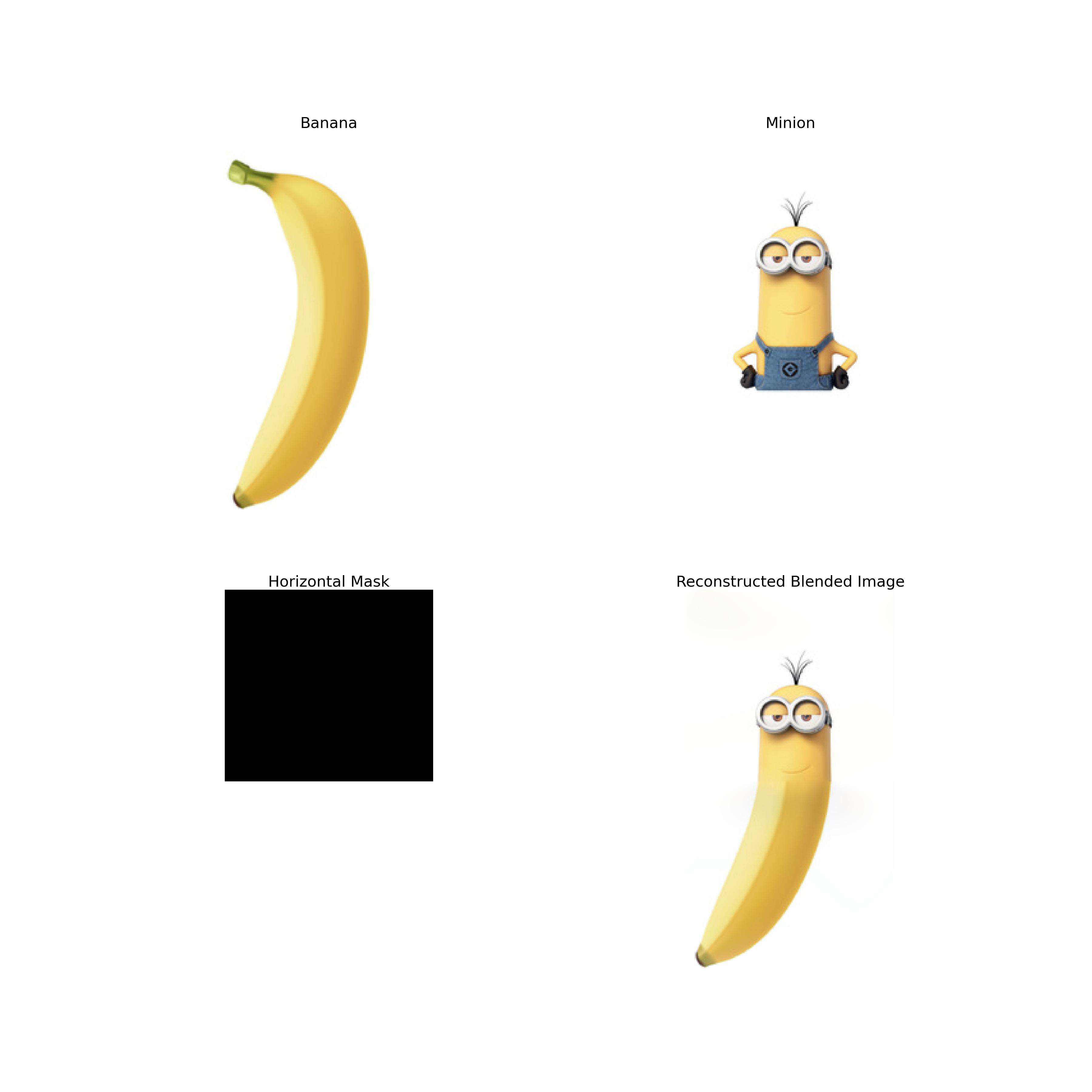
The image above shows the result of blending a banana and a minion using multi-resolution blending.
The image above is the hybrid image of a mango and the Hongwu Emperor (whose portrait looks like a mango).
This part explores the use of finite difference operators to compute the gradient of an image. The gradient is computed using two filters: dx and dy. The dx filter computes the gradient in the x-direction, while the dy filter computes the gradient in the y-direction.
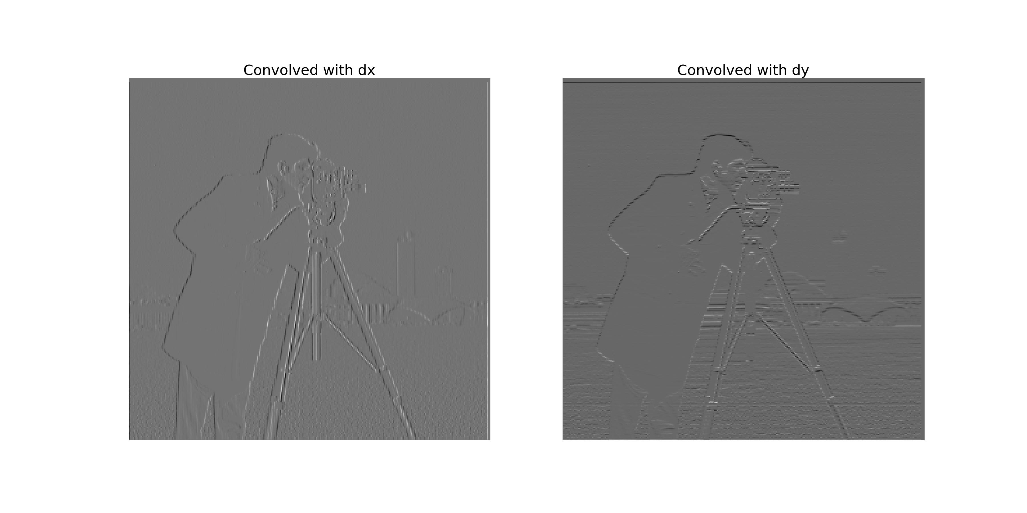
The image above shows the results of convolving the cameraman image with the dx and dy filters.
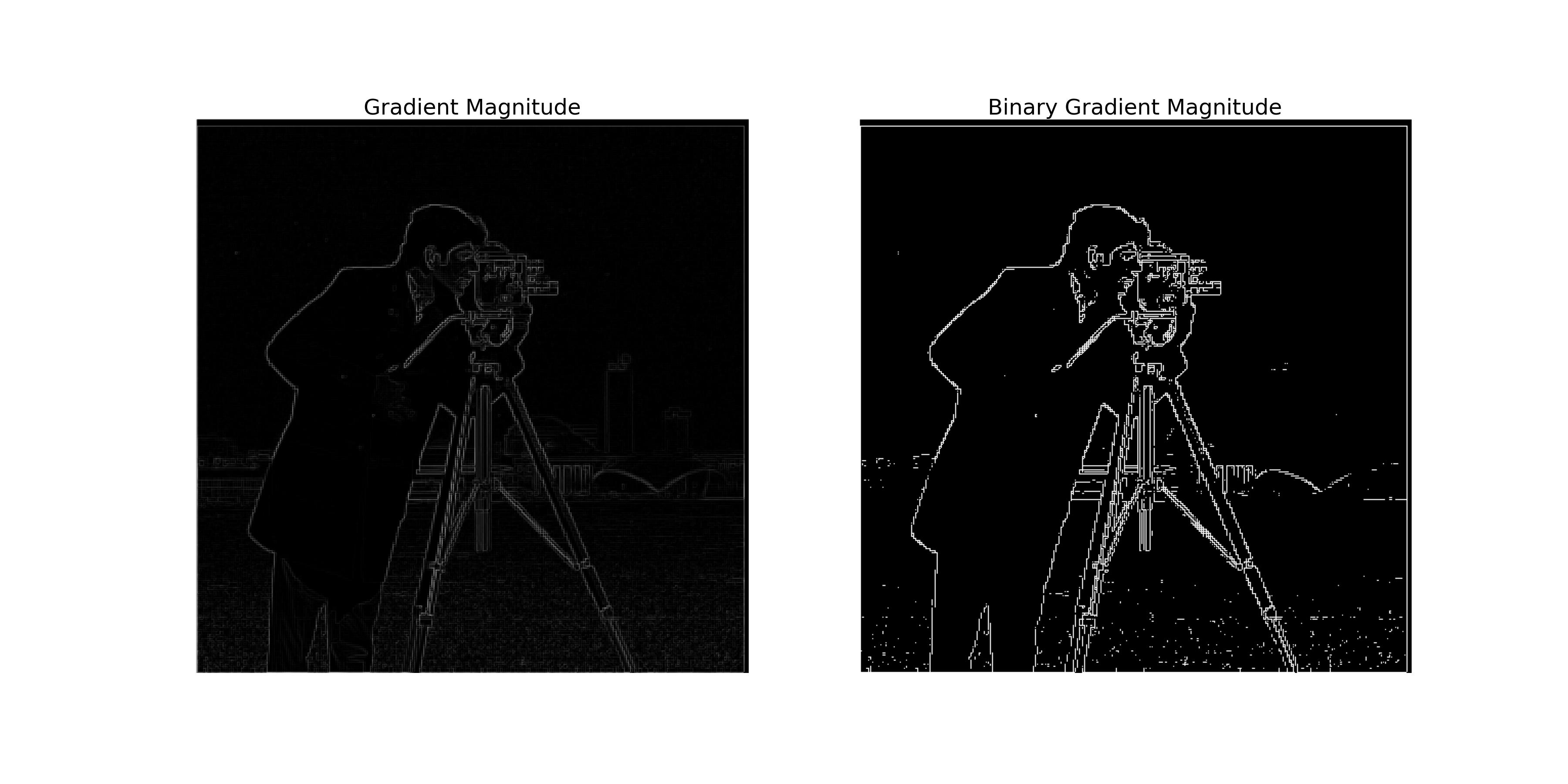
The image above shows the gradient magnitude of the cameraman image.
This part explores the use of the derivative of Gaussian (DoG) filter to compute the gradient of an image. The DoG filter is a combination of a Gaussian filter and a derivative filter. The Gaussian filter is used to smooth the image, while the derivative filter is used to compute the gradient.
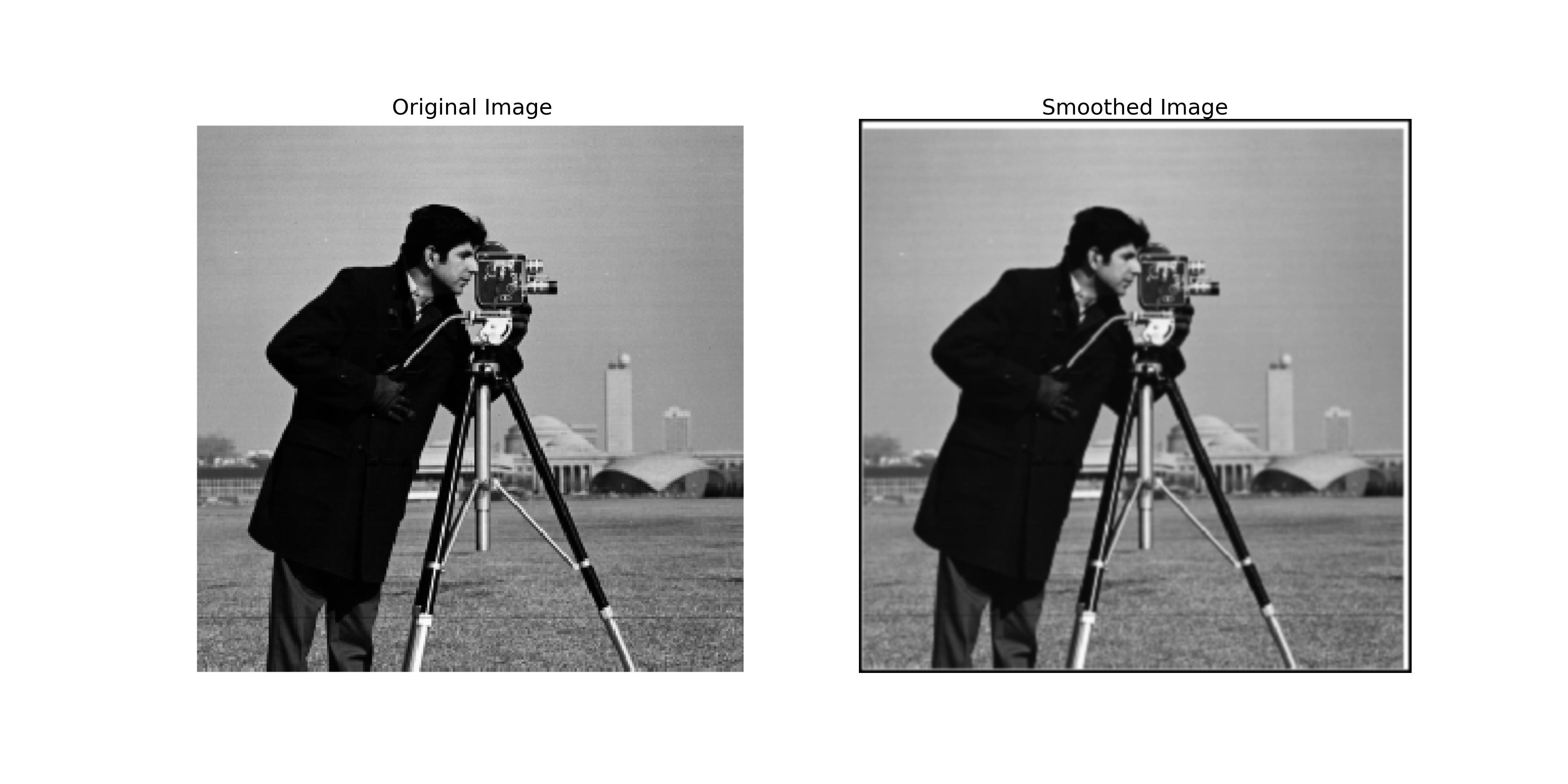
The image above shows the result of convolving the cameraman image with the Gaussian filter.
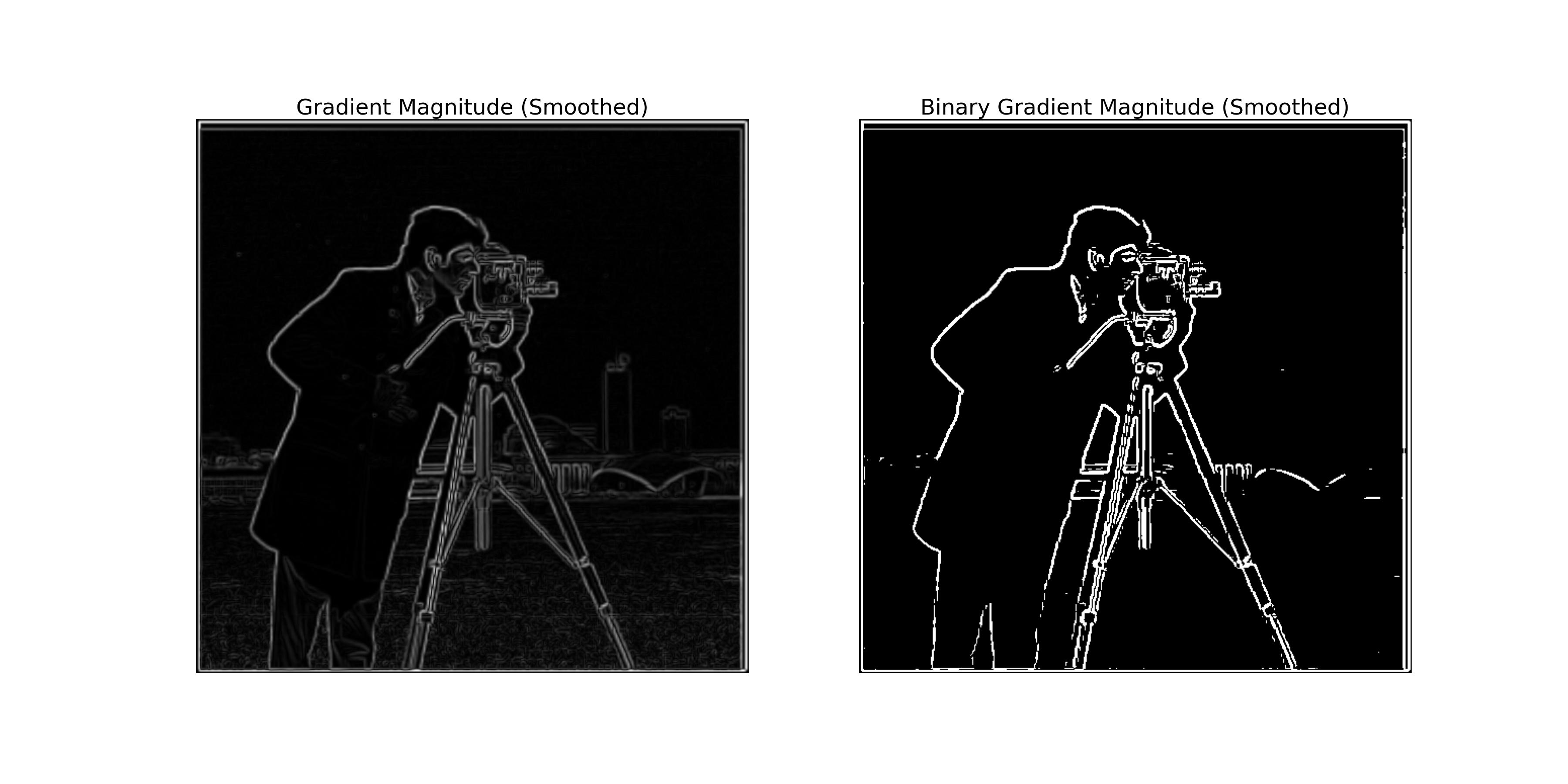
The image above shows the gradient magnitude of the smoothed cameraman image.
By comparing the results of the finite difference operator and the DoG filter, we can see the following differences:
We can combine the Gaussian filter and the derivative filter into a single filter called the DoG filter.
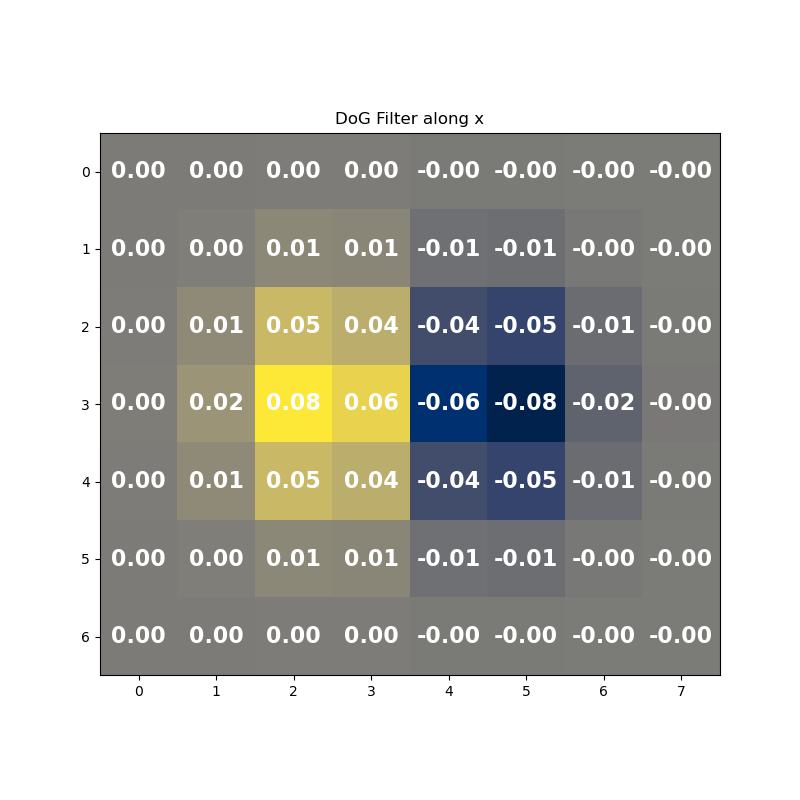
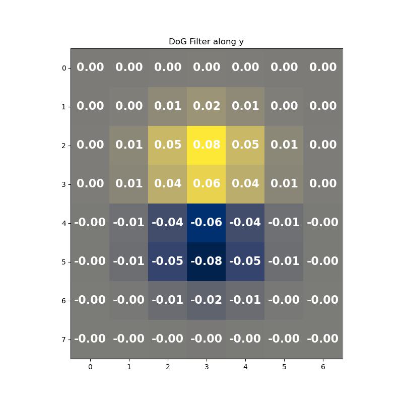
The images above show the DoG filters in the x-direction and y-direction.
We can convolve the cameraman image with the DoG filters directly to compute the gradient after smoothing the image. The following images show the results of convolving the cameraman image directly with the DoG filters is the same as convolving the smoothed image with the finite difference operator.
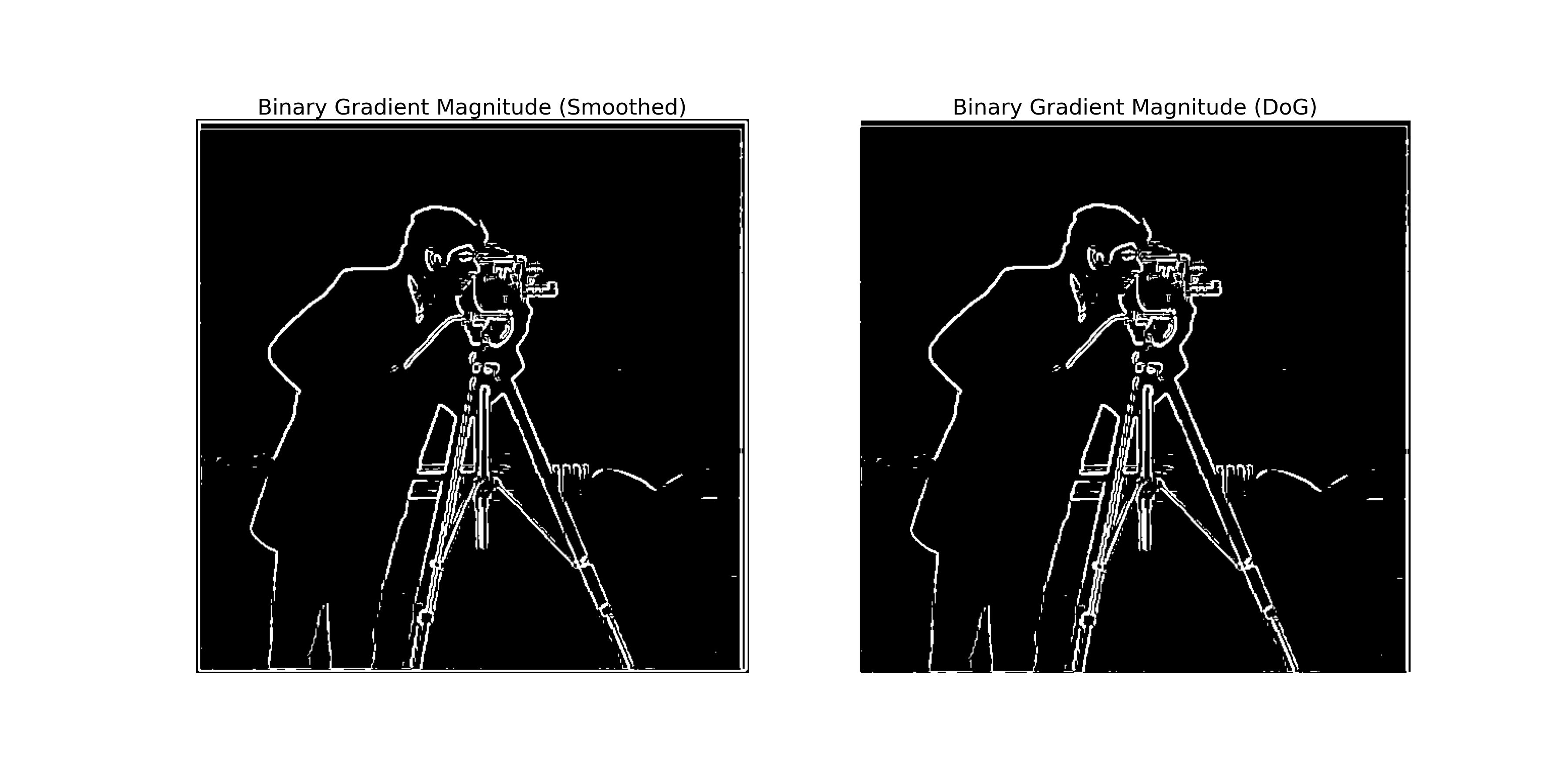
The left image above is the gradient magnitude of the smoothed cameraman image convolved with the gradient filters. The right image above is the gradient magnitude of the cameraman image convolved with the DoG filters.
This part explores the use of unsharp masking technique to sharpen an image. The unsharp masking technique involves subtracting a blurred version of the image from the original image to enhance the edges. We can derive the unsharp masking filter by subtracting the Gaussian filter from the unit impulse filter. \[ \text{{unsharp\_masking\_filter}} = (1 + \alpha) \times \text{{unit\_impulse\_filter}} - \alpha \times \text{{gaussian\_filter}} \] where \(\alpha\) is a parameter that controls the strength of the sharpening effect.
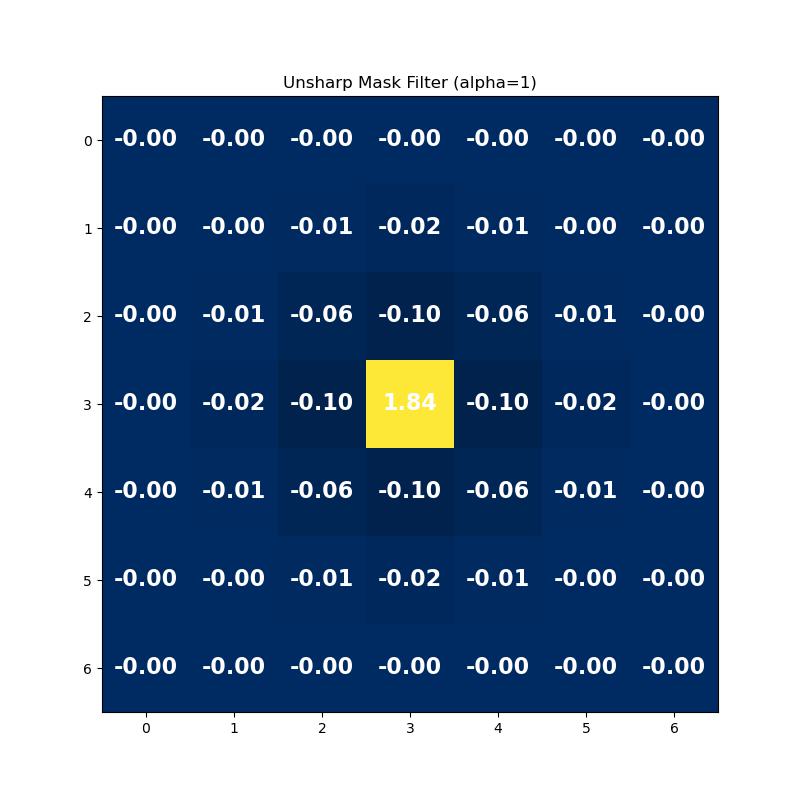
The image above shows the unsharp masking filter with alpha = 1.
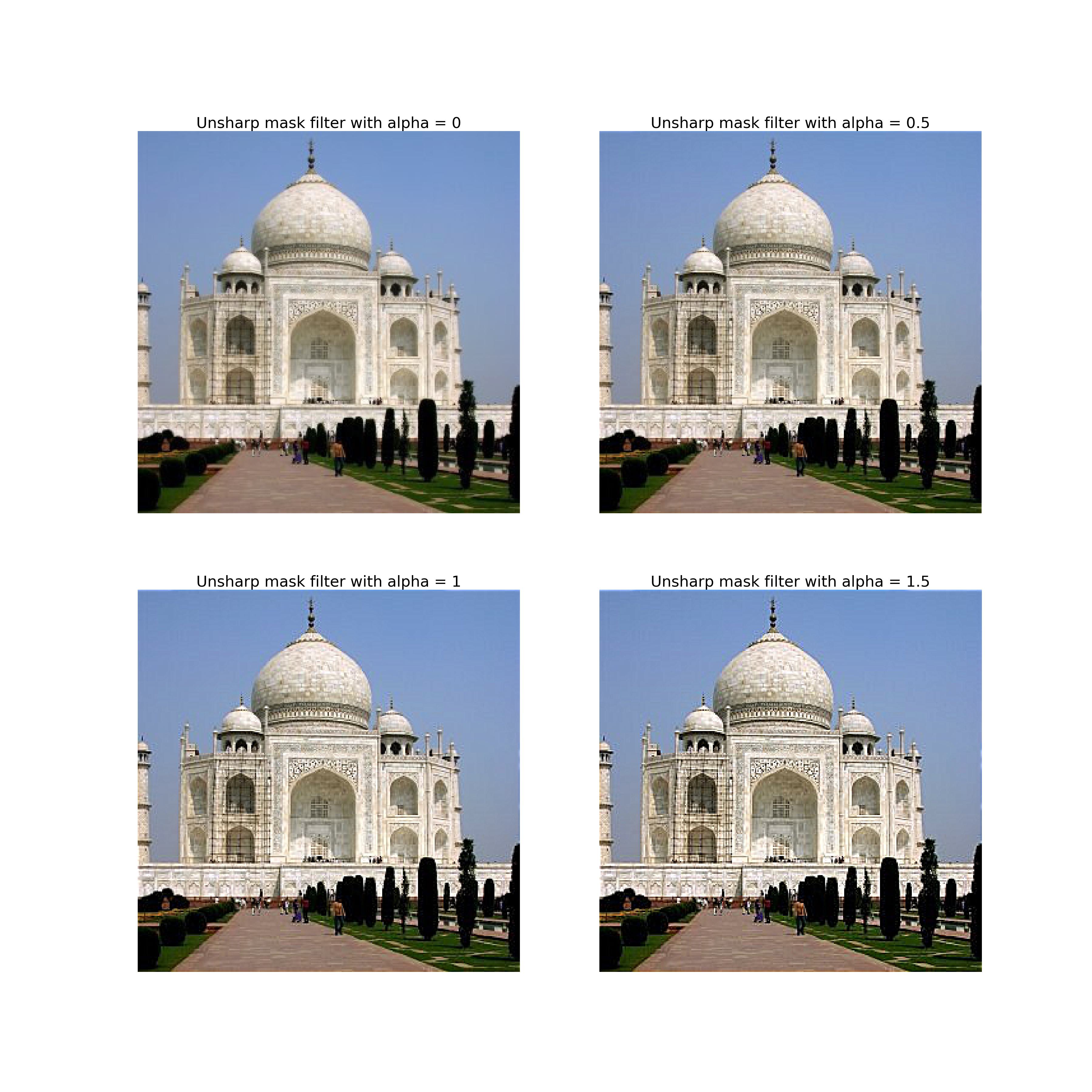
The image above shows the results of sharpening the Taj image with the unsharp masking filter of different alphas.
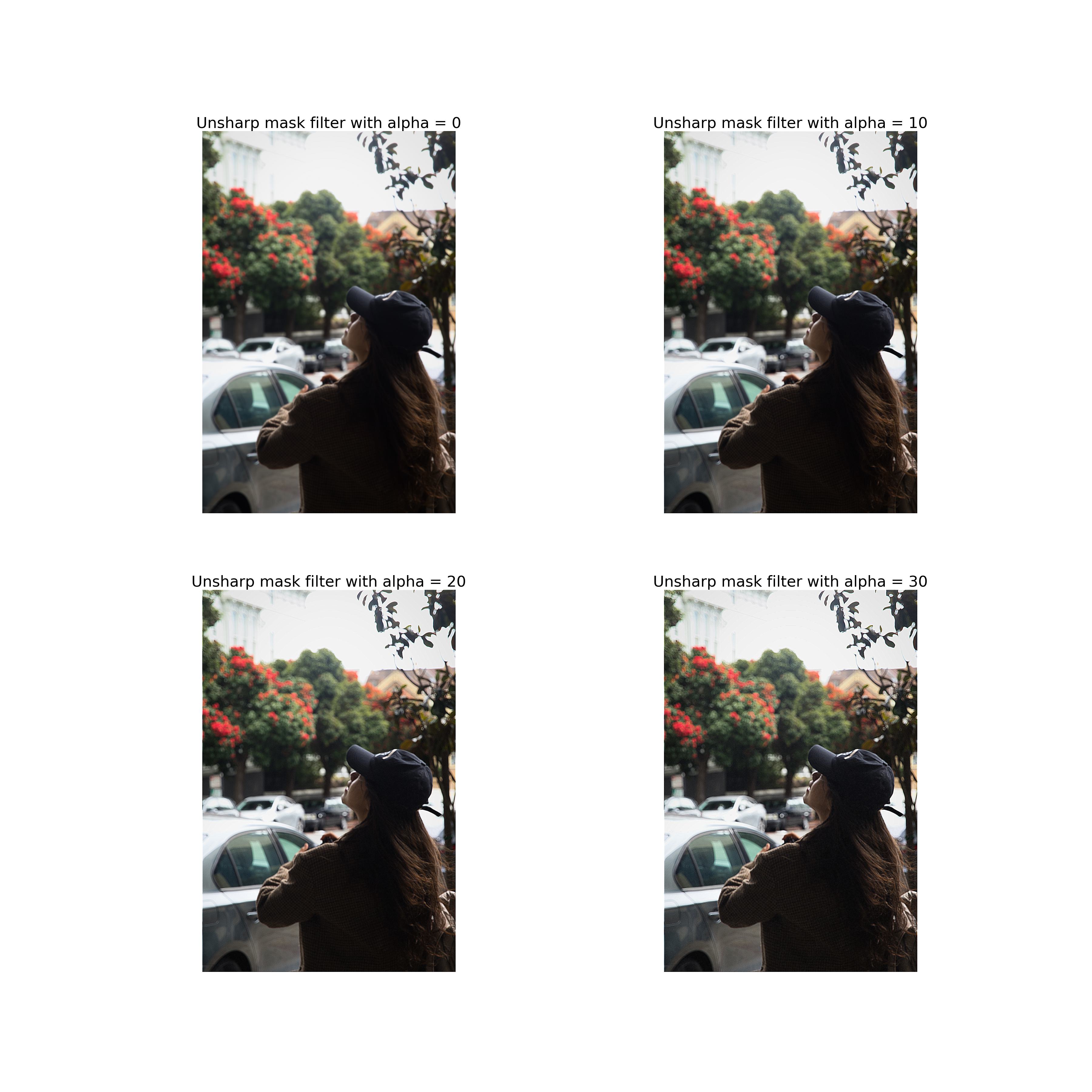
The image above shows the results of sharpening a out of focus image with the unsharp masking filter of different alphas. We can see that after sharpening, the edges become more pronounced and the details become clearer. However, the sharpening effect can also enhance noise and artifacts in the image.
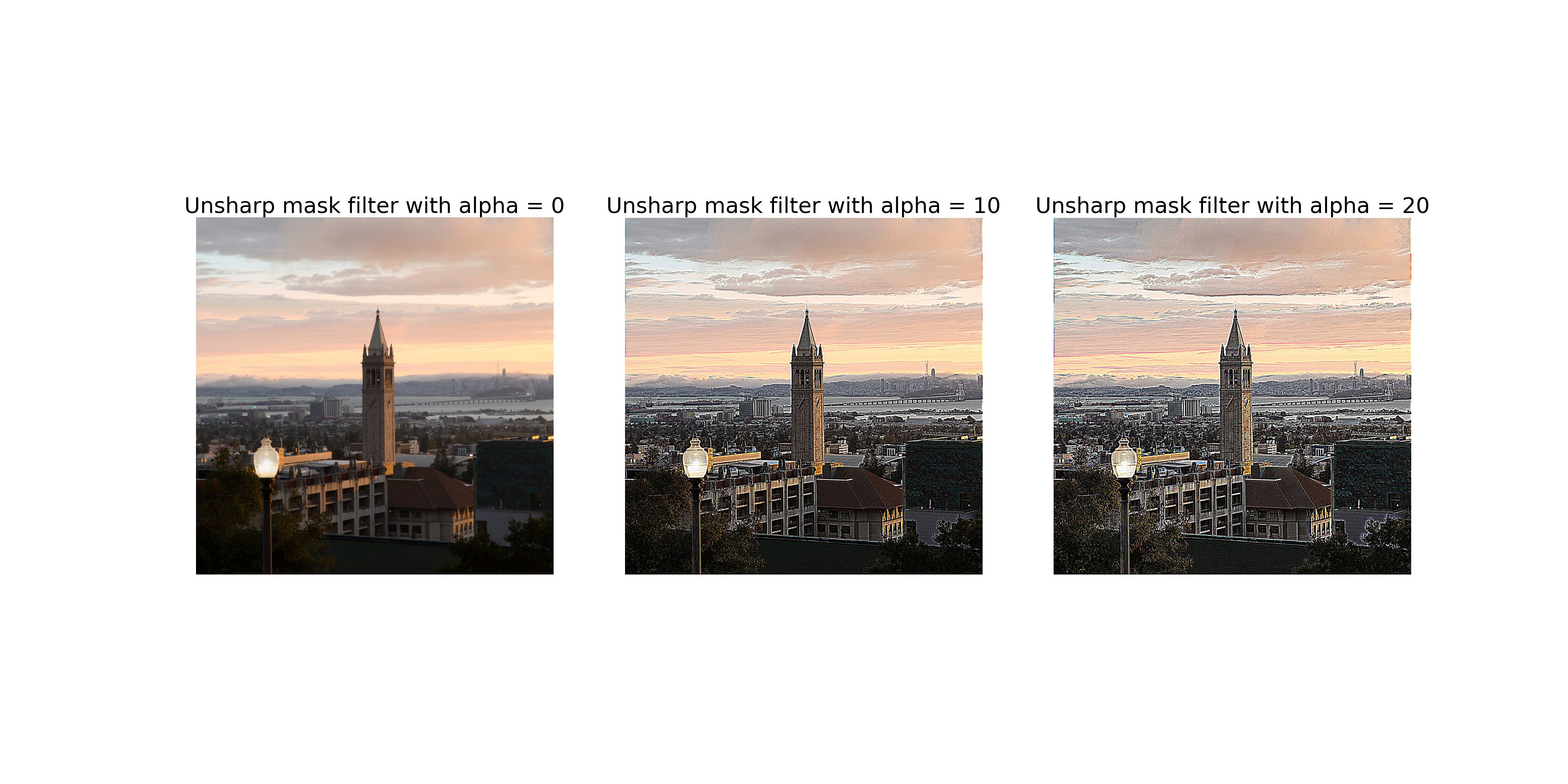
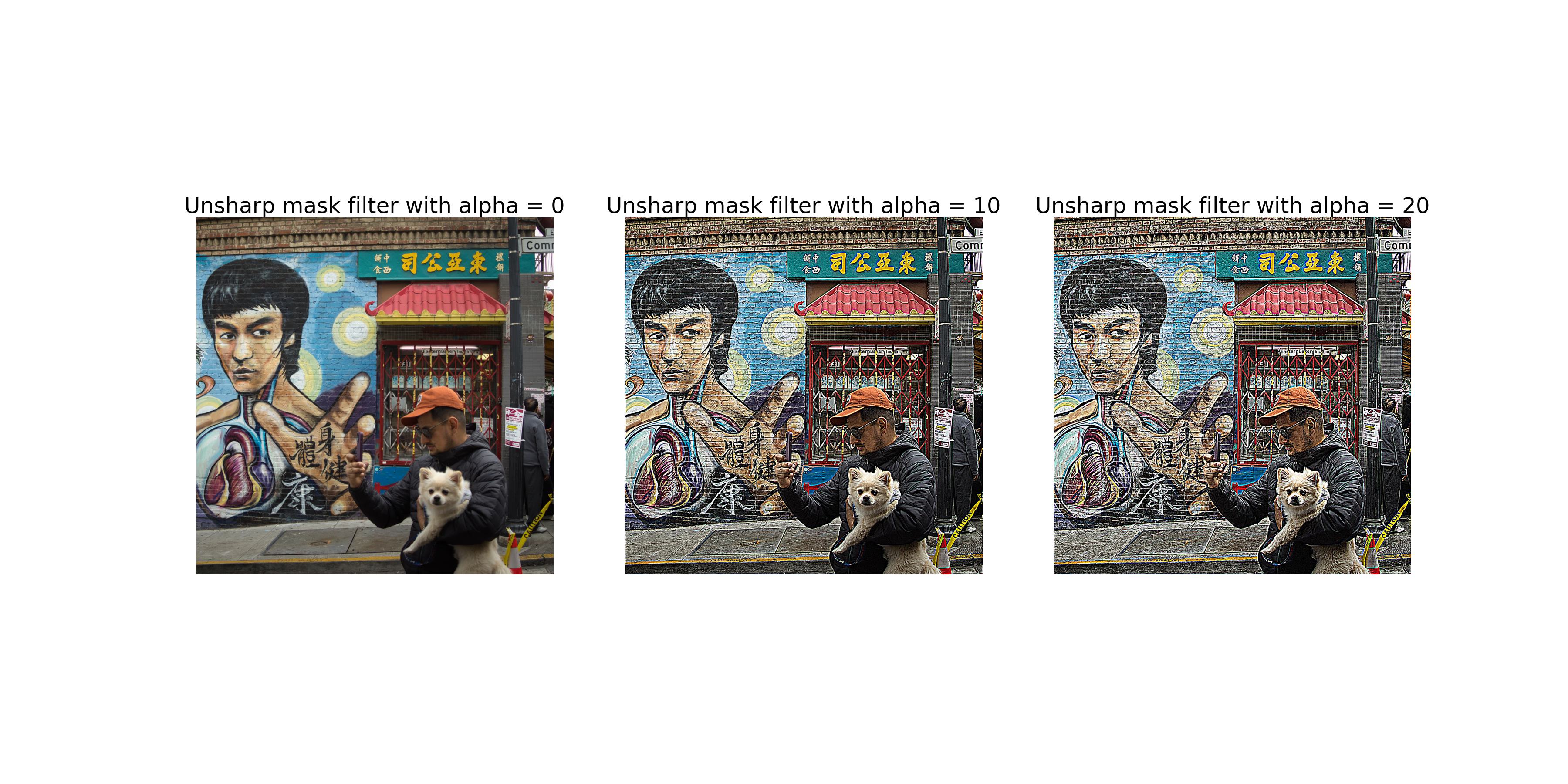
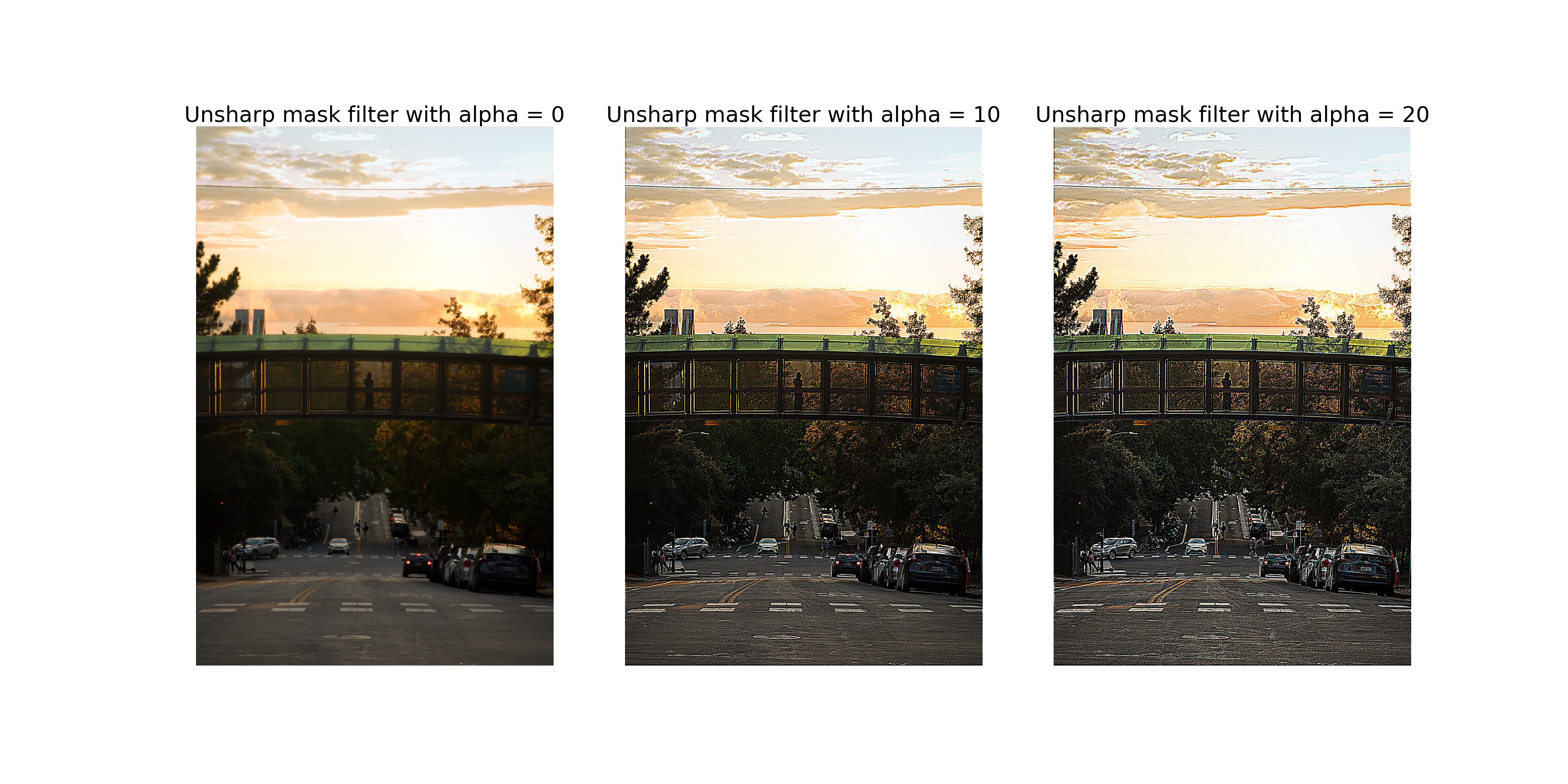
Some other photos taken by me are also sharpened using the unsharp masking filter. The results are shown below.
The results of blurring a sharp image and then sharpening it are shown below.
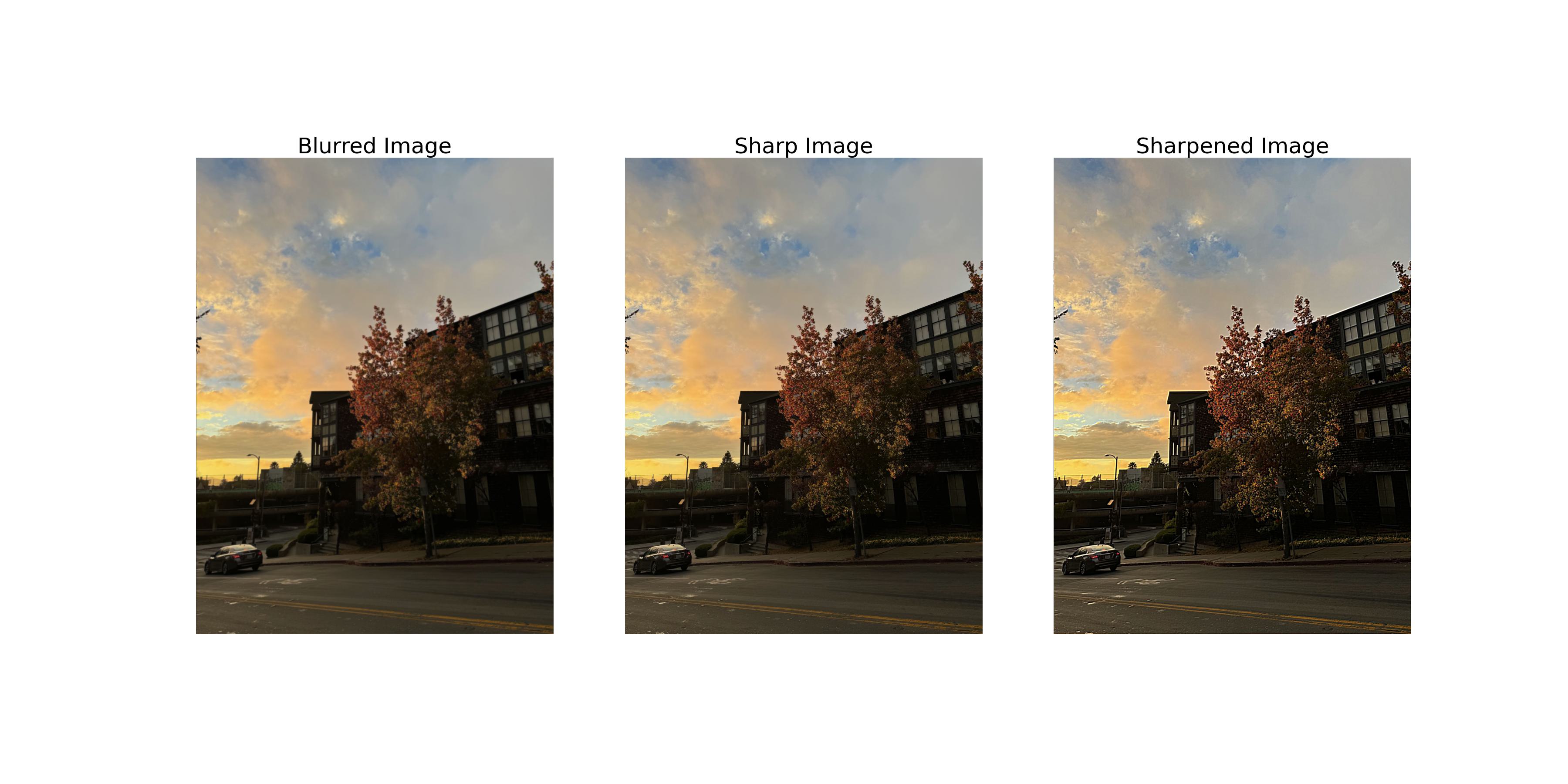
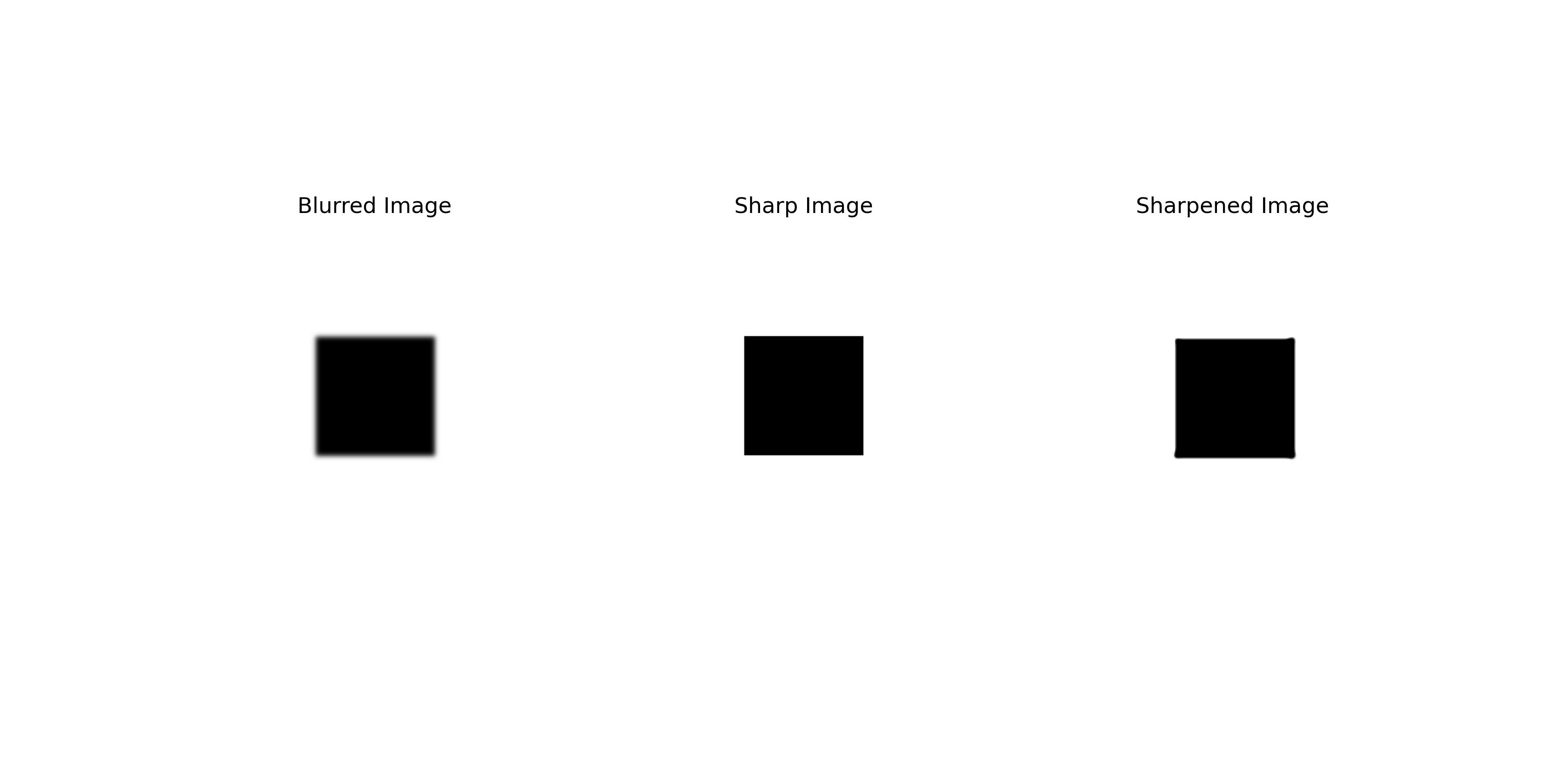
Although the sharpened image is sharper than the blurred image, it is still different from the original image in the following ways:
This part explores the creation of hybrid images by combining the low-frequency components of one image with the high-frequency components of another image. The low-frequency components are obtained by applying a Gaussian filter to the first image, while the high-frequency components are obtained by subtracting the Gaussian-filtered image from the original image.
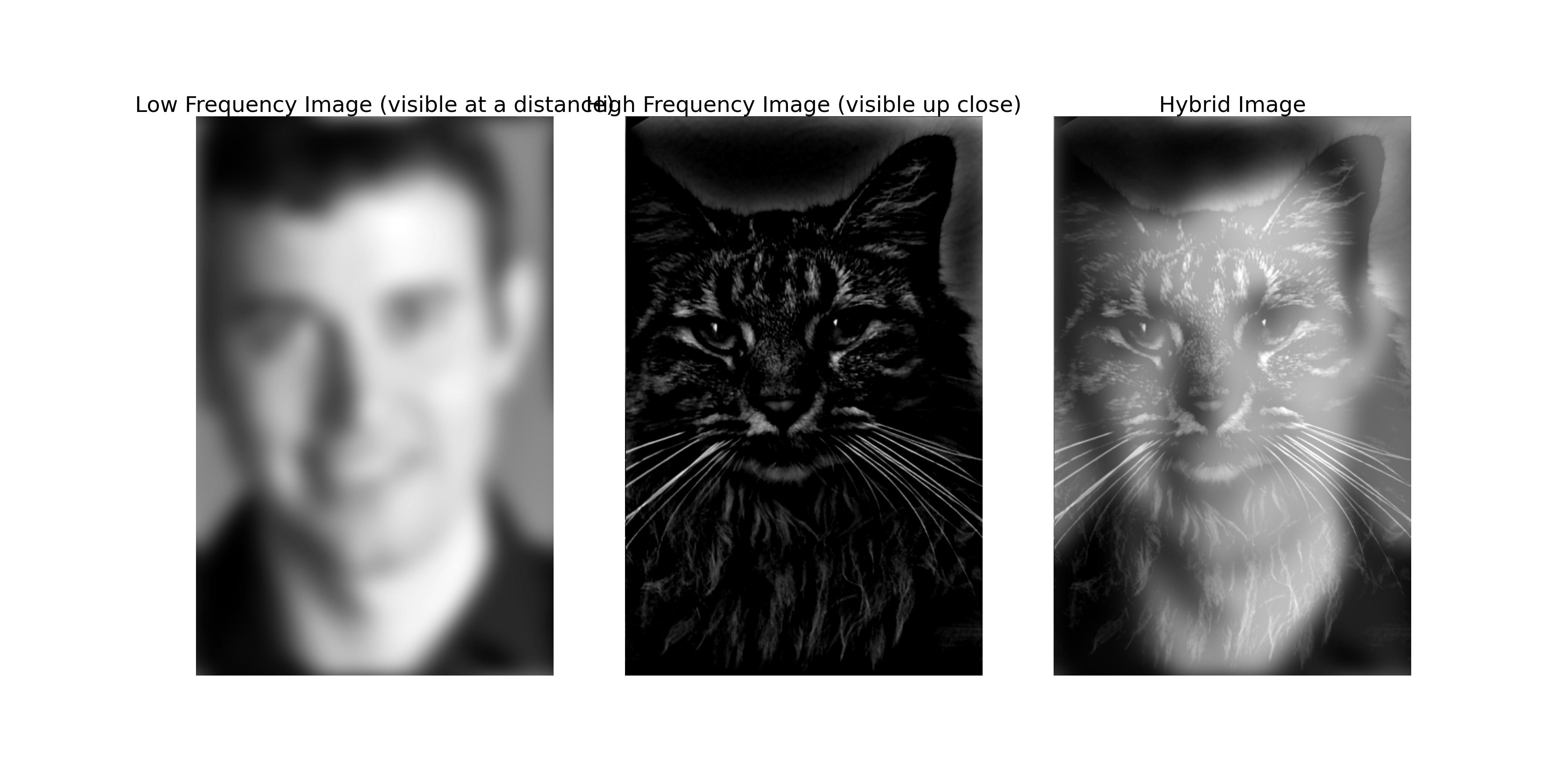
The image above shows the sample hybrid image of a cat and a man. The low-frequency components of the man image are combined with the high-frequency components of the cat image to create the hybrid image.
The Hongwu Emperor (1328-1398) of the Ming Dynasty is known for his distinctive appearance, which some say resembles a mango 🤣.

The images above show the aligned images of the mango and the Hongwu Emperor and the hybrid image of the two images.
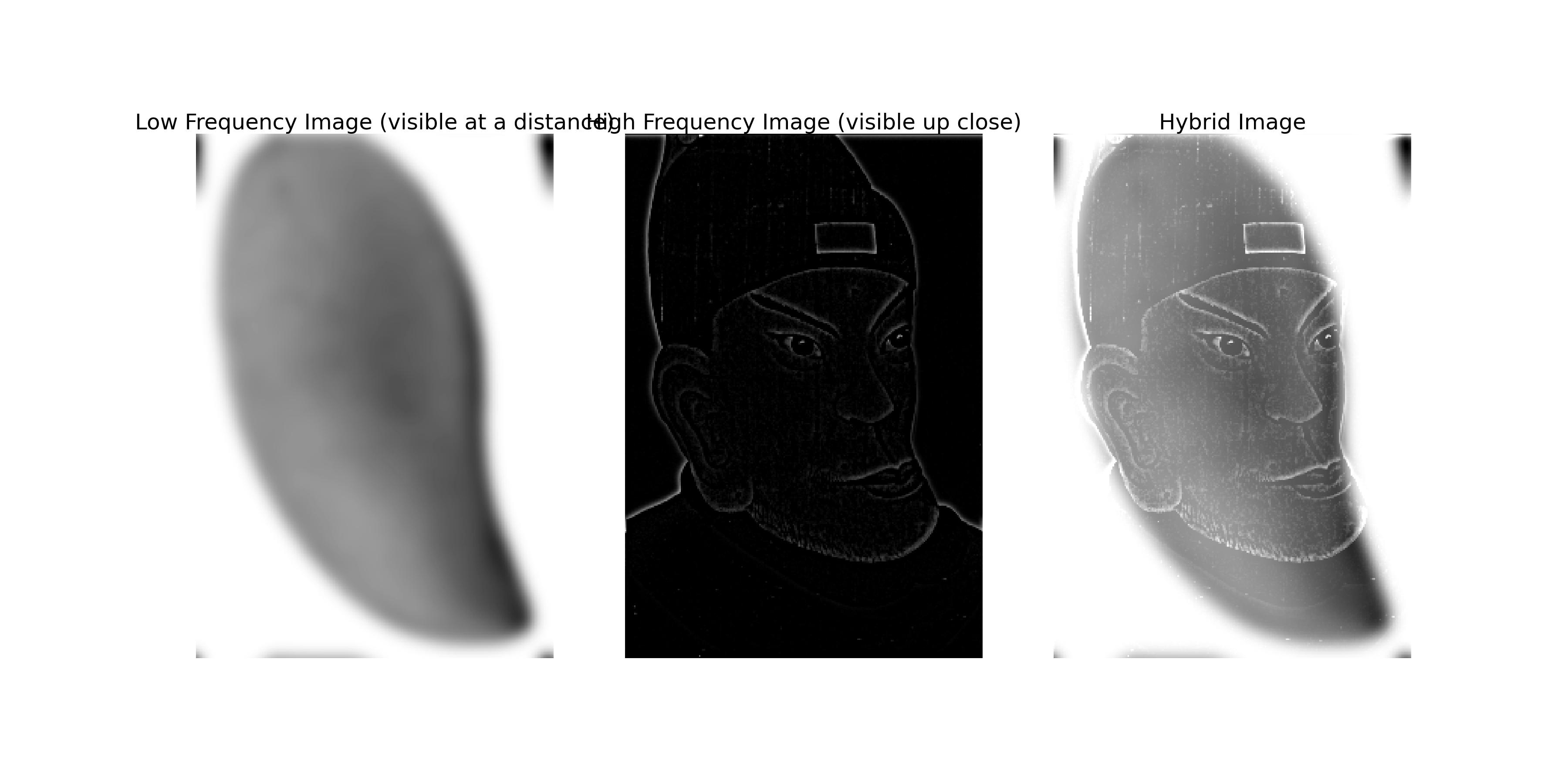
The image above shows the hybrid image of the mango and the Hongwu Emperor. The low-frequency components of the mango image are combined with the high-frequency components of the Hongwu Emperor image to create the hybrid image.
We can conduct some frequency analysis on the hybrid image to understand how the low-frequency and high-frequency components are combined. The following images are the log magnitude of the Fourier transform of the mango image, the Hongwu Emperor image, and the hybrid image.
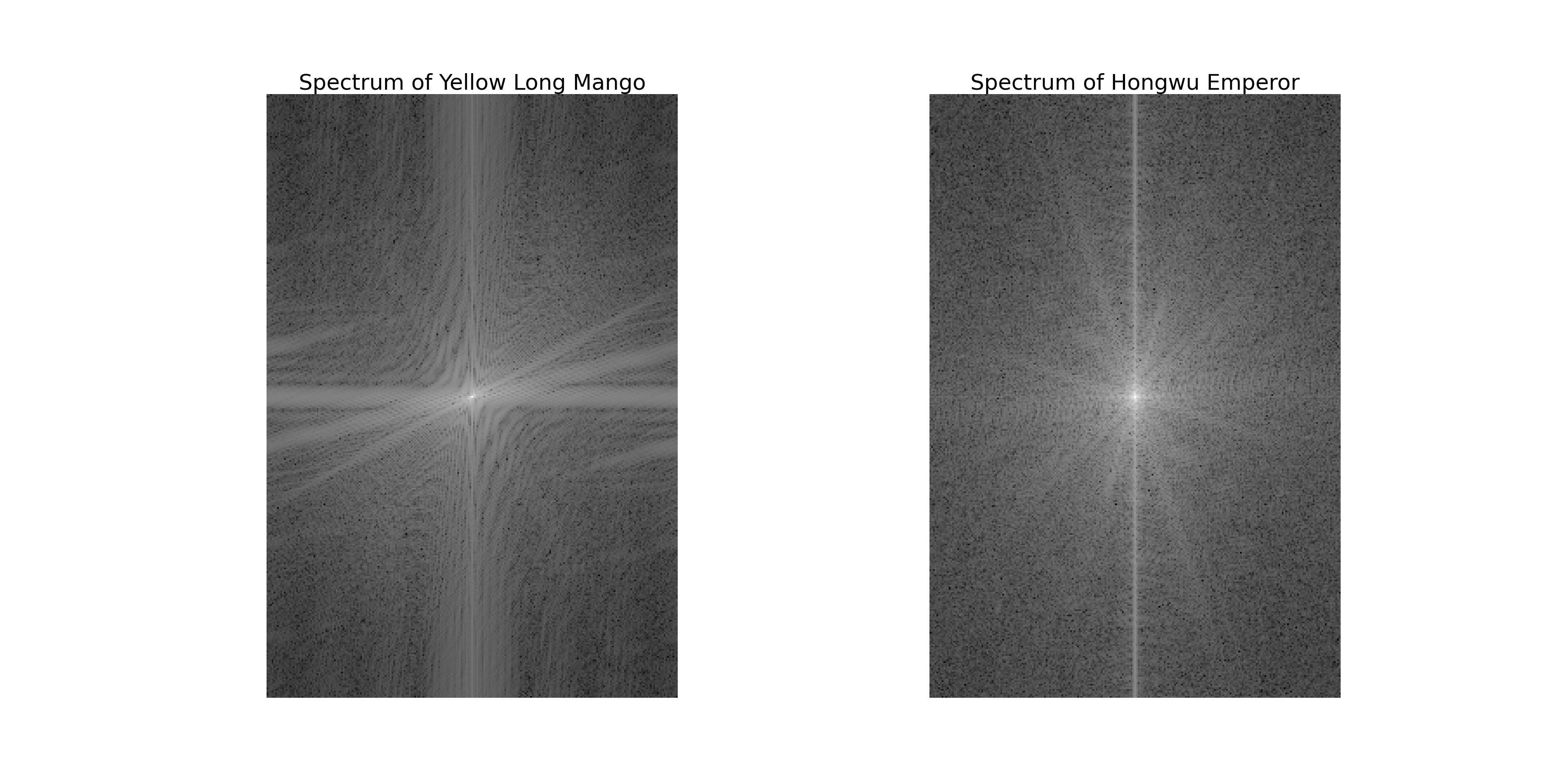
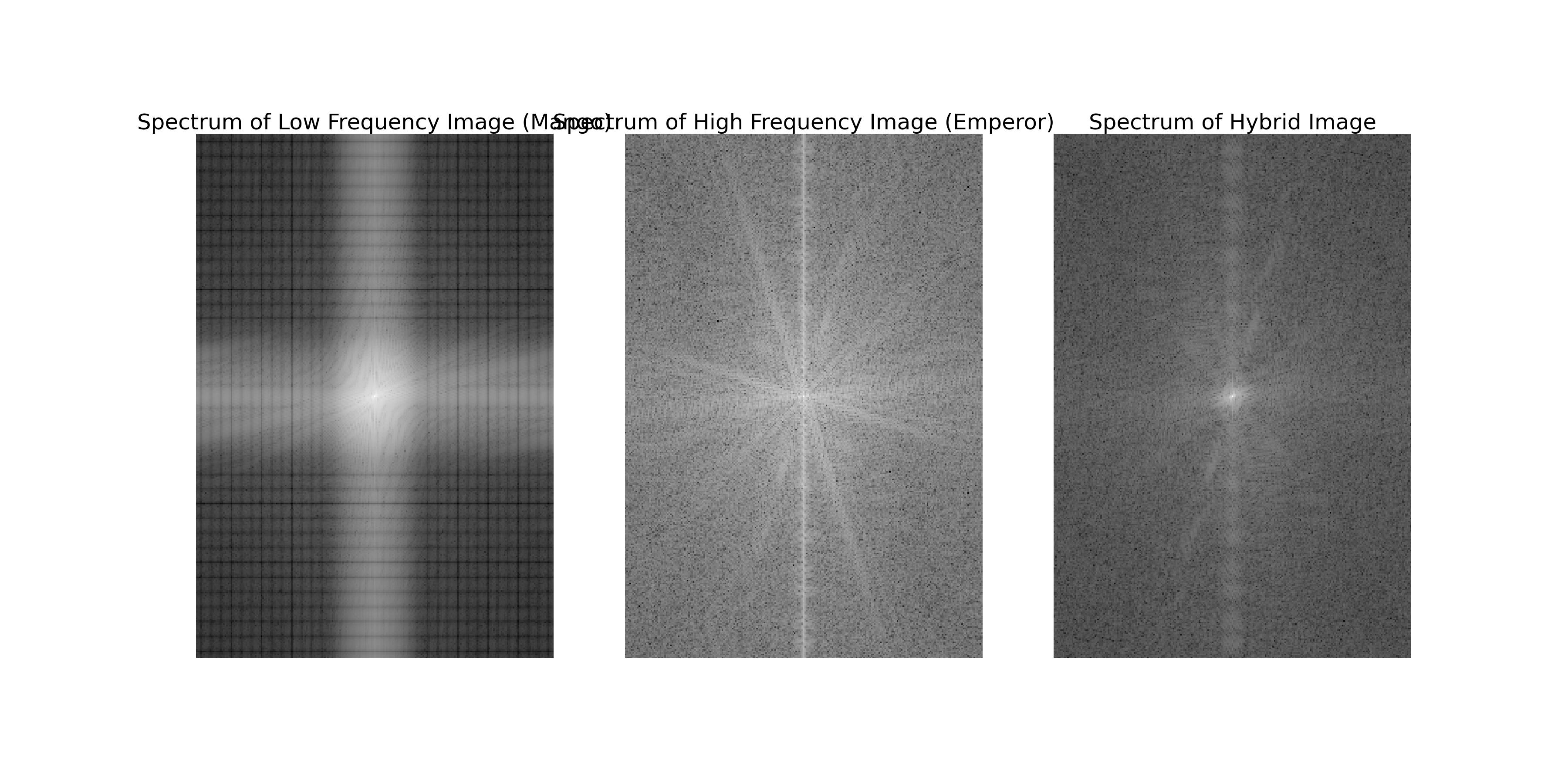
We can see that the mango image after low-pass filtering has less high-frequency components, while the Hongwu Emperor image after high-pass filtering has more high-frequency components. The hybrid image combines the low-frequency components of the mango image with the high-frequency components of the Hongwu Emperor image.
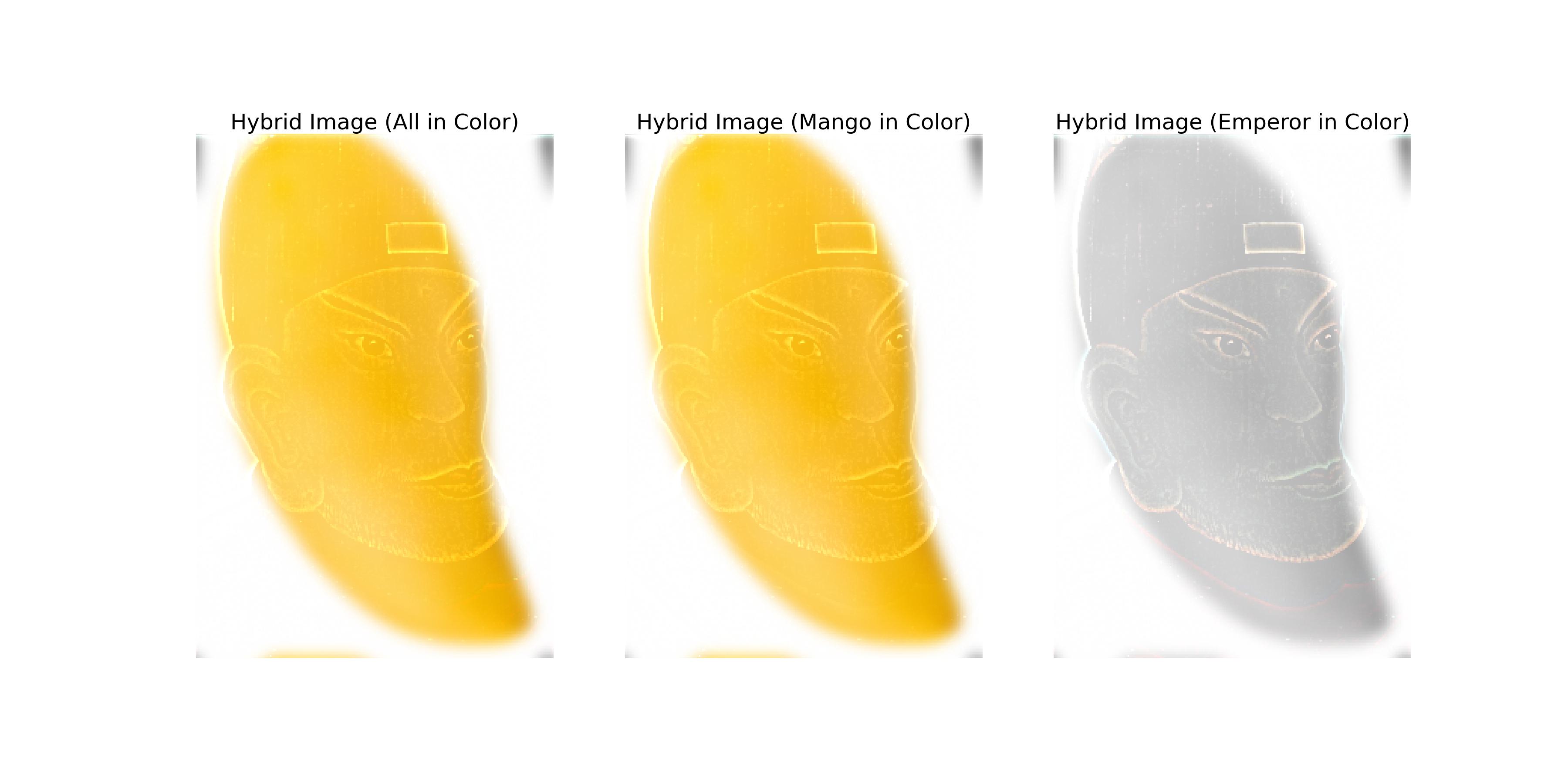
The hybrid image can also be created in color by retaining any color information in the two images. The following image shows the hybrid image of the mango and the Hongwu Emperor in color.

The left image above retains the color information of both images. The middle image above retains the color information of the mango image. The right image above retains the color information of the Hongwu Emperor image.
After trying different color combinations, I found that the best color combination for enhancing the effect of the hybrid image is to use the color of the high-frequency image as the color of the hybrid image while keeping the low-frequency image in grayscale.
I think the main reason for this is that a common problem with hybrid images is that the low-frequency image is often too dominant, and using color on the high-frequency image helps to make the high-frequency image more prominent at a closer distance while still allowing the low-frequency image to be visible at a farther distance.
Shenzhen is my hometown, and it has undergone significant changes over the past few decades. The following images are the aligned images of Shenzhen in 1982 and 2018.
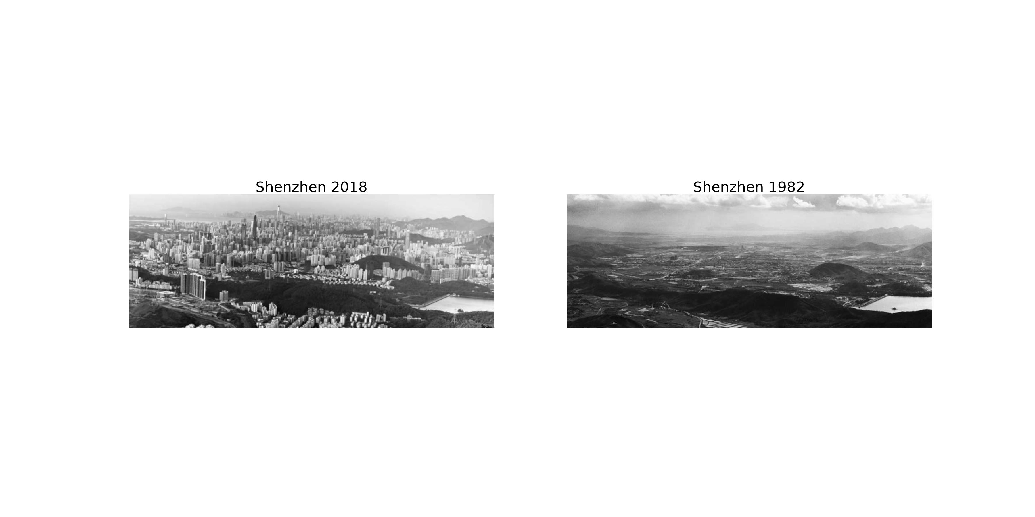
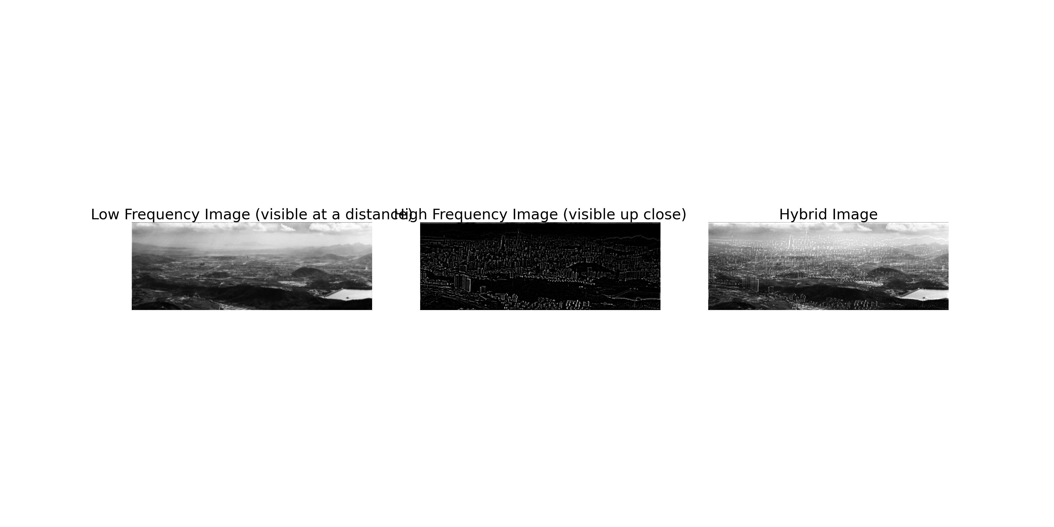
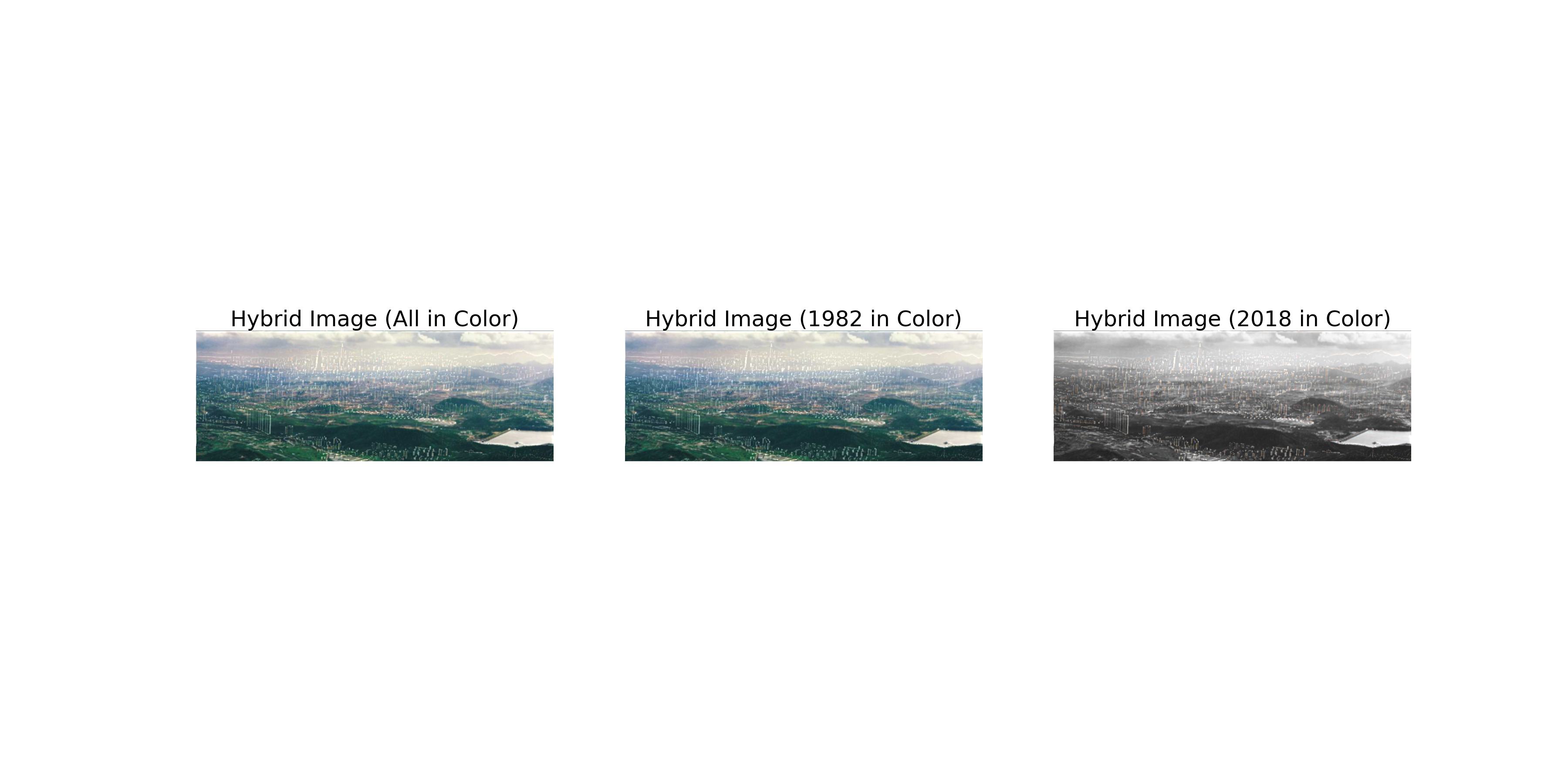
The following images show the hybrid images of Shenzhen in 1982 and 2018. The low-frequency components of the 1982 image are combined with the high-frequency components of the 2018 image to create the hybrid image.
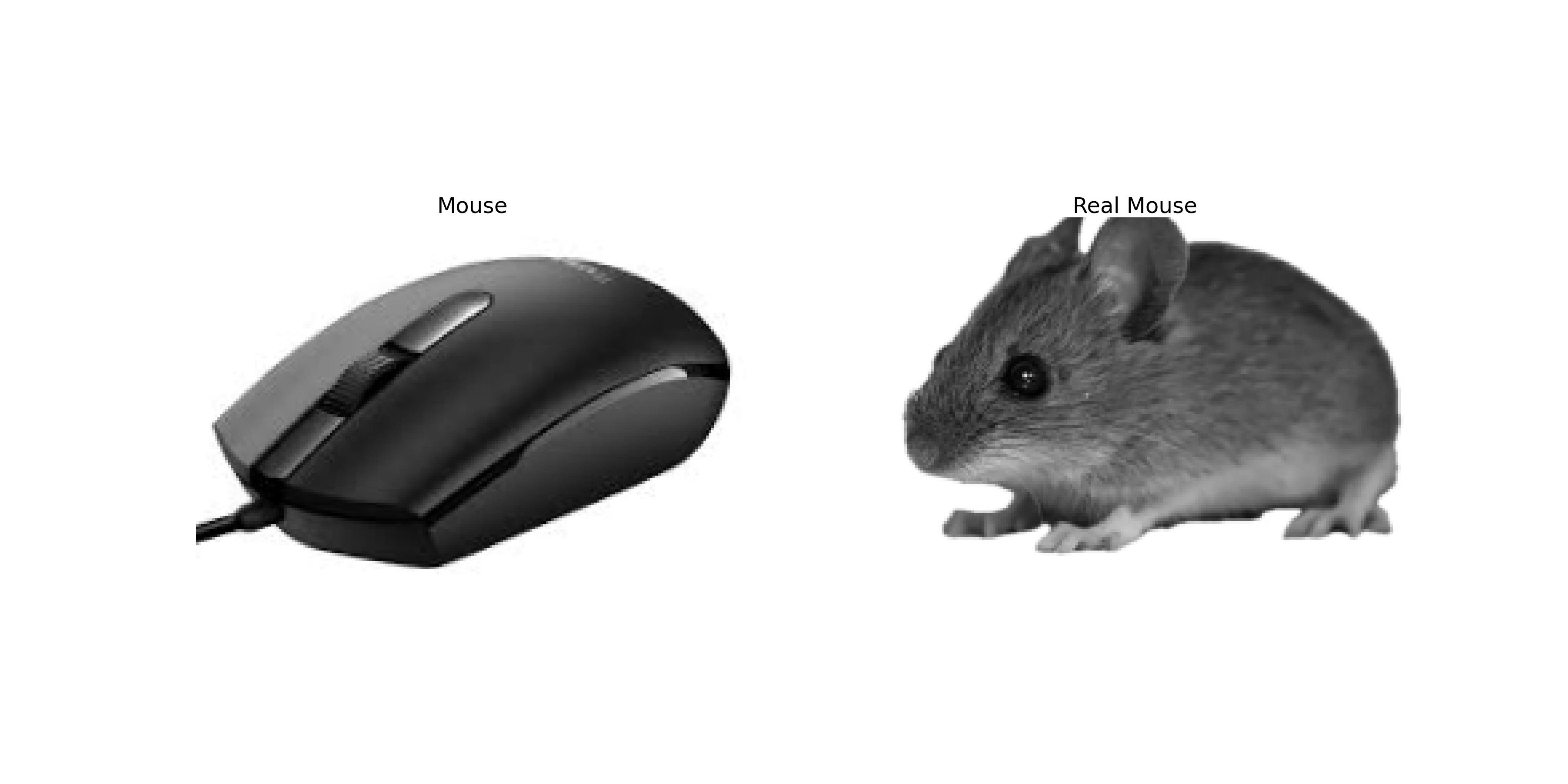
Why is it called a computer mouse? Are there any similarities between a mouse and a computer mouse? The following images are the aligned images of a mouse and a computer mouse.
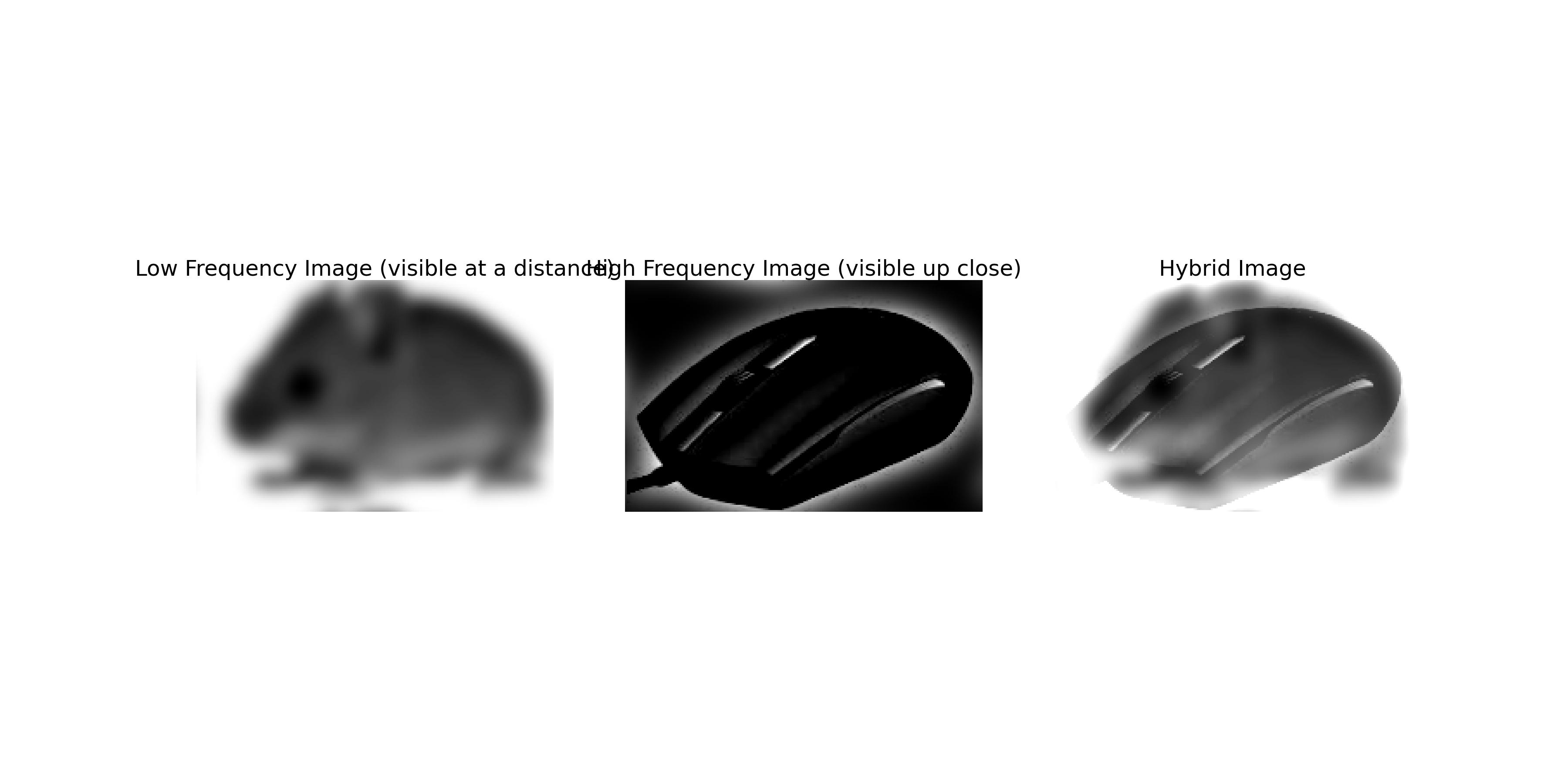
The following images show the hybrid images of a mouse and a computer mouse. The low-frequency components of the mouse image are combined with the high-frequency components of the computer mouse image to create the hybrid image.
This part explores the creation of Gaussian and Laplacian stacks for multi-resolution blending. The Gaussian stack is created by applying a series of Gaussian filters to the original image, while the Laplacian stack is created by subtracting the Gaussian-filtered image from the original image.
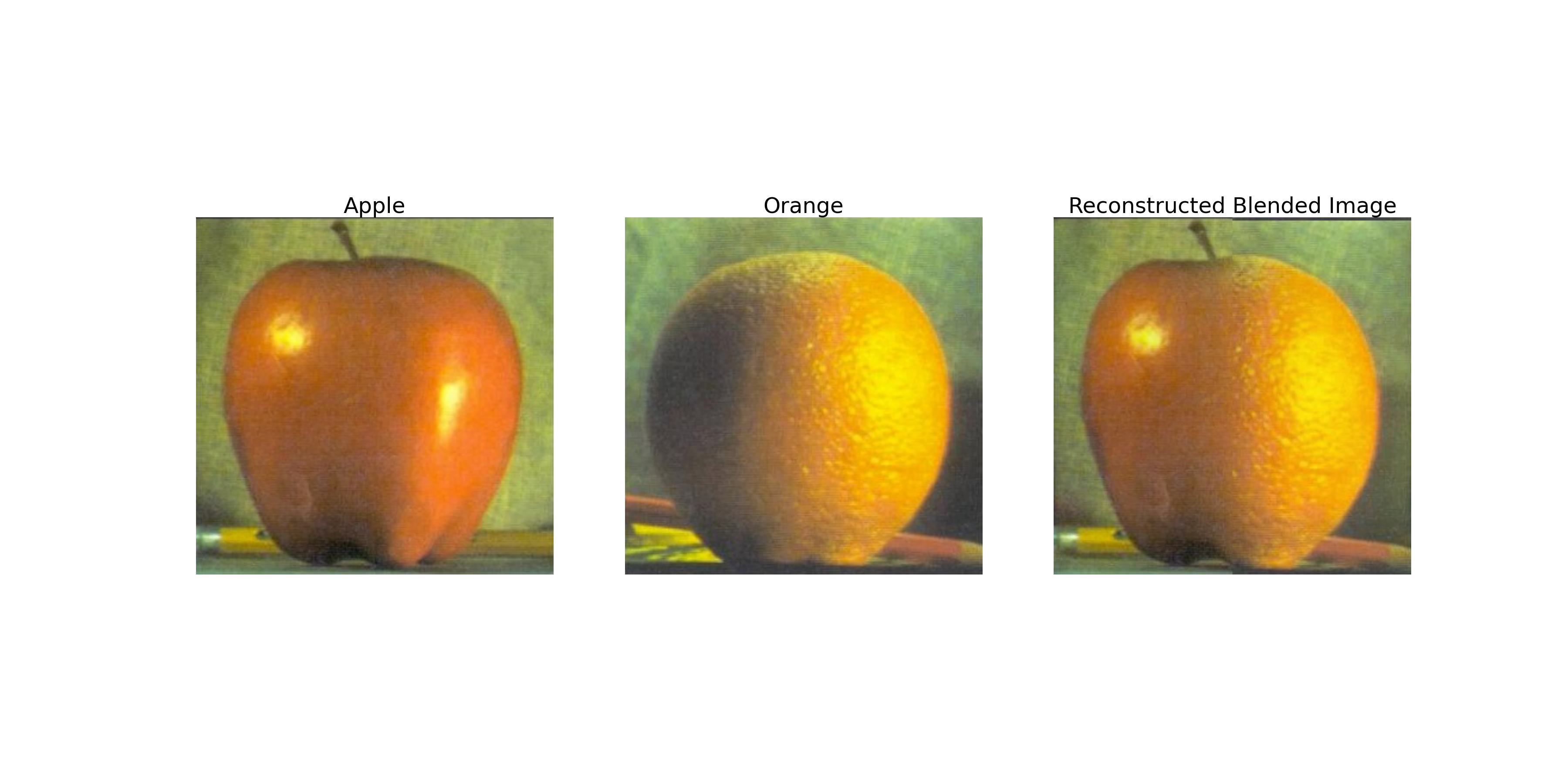
The image above shows the result of blending an apple and an orange using multi-resolution blending. I used \(\sigma = 3\) for the Gaussian filter and 50 levels for the Gaussian and Laplacian stacks.
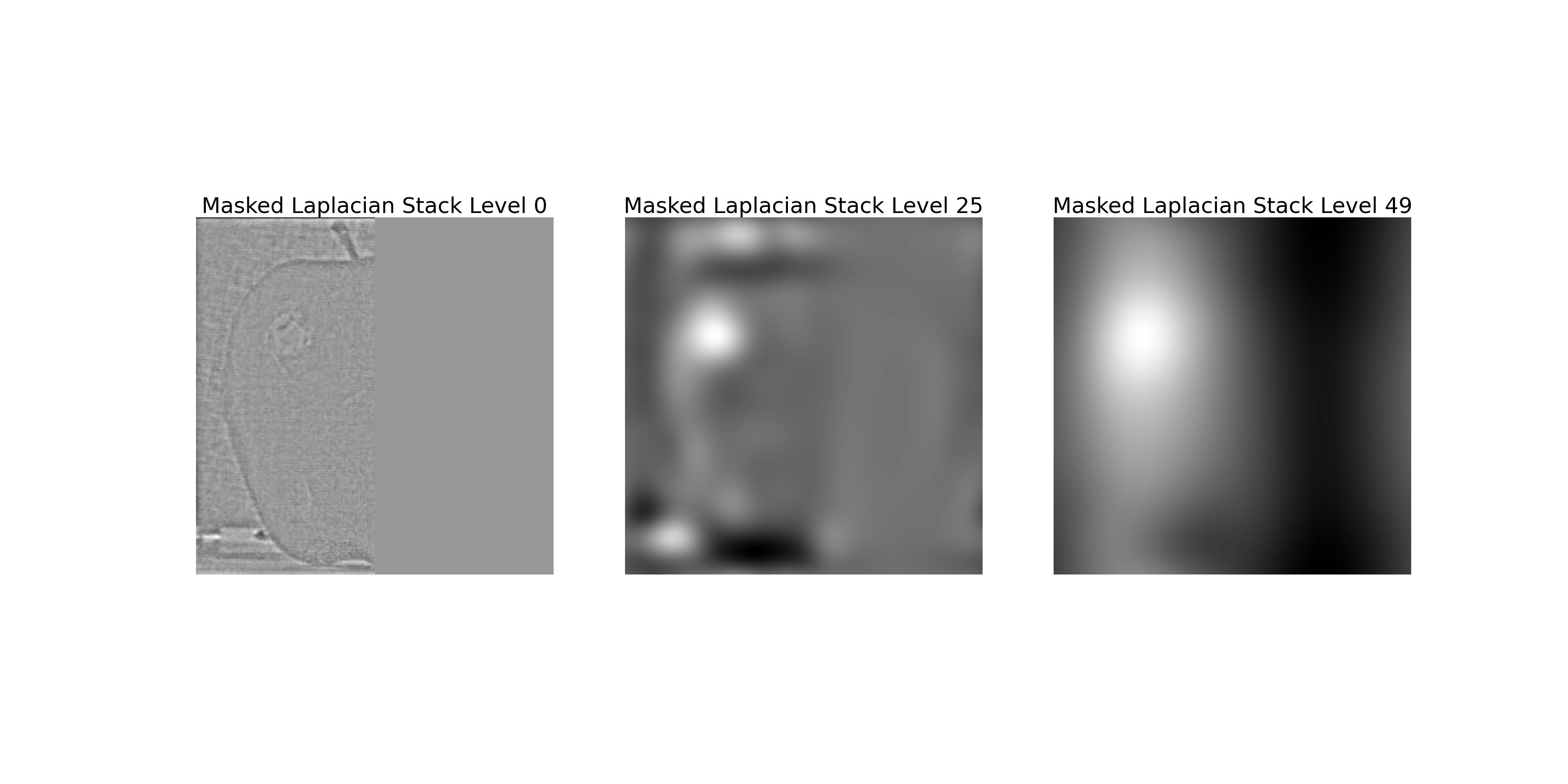
The image above shows the Laplacian stack of the apple image with the mask applied to each level. This corresponds to the left column of Figure 3.42 in the textbook.
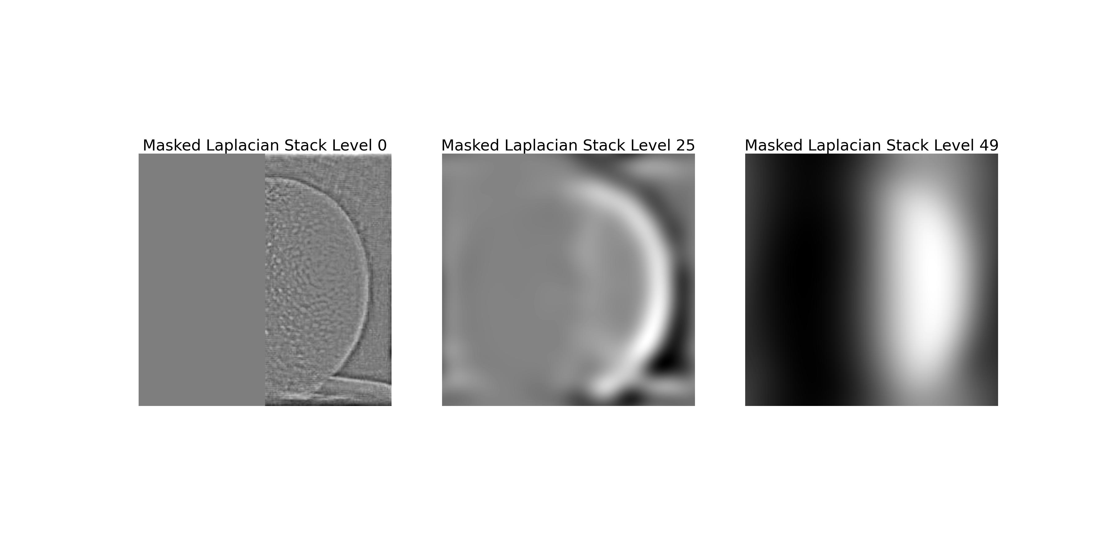
The image above shows the Laplacian stack of the orange image with the mask applied to each level. This corresponds to the middle column of Figure 3.42 in the textbook.
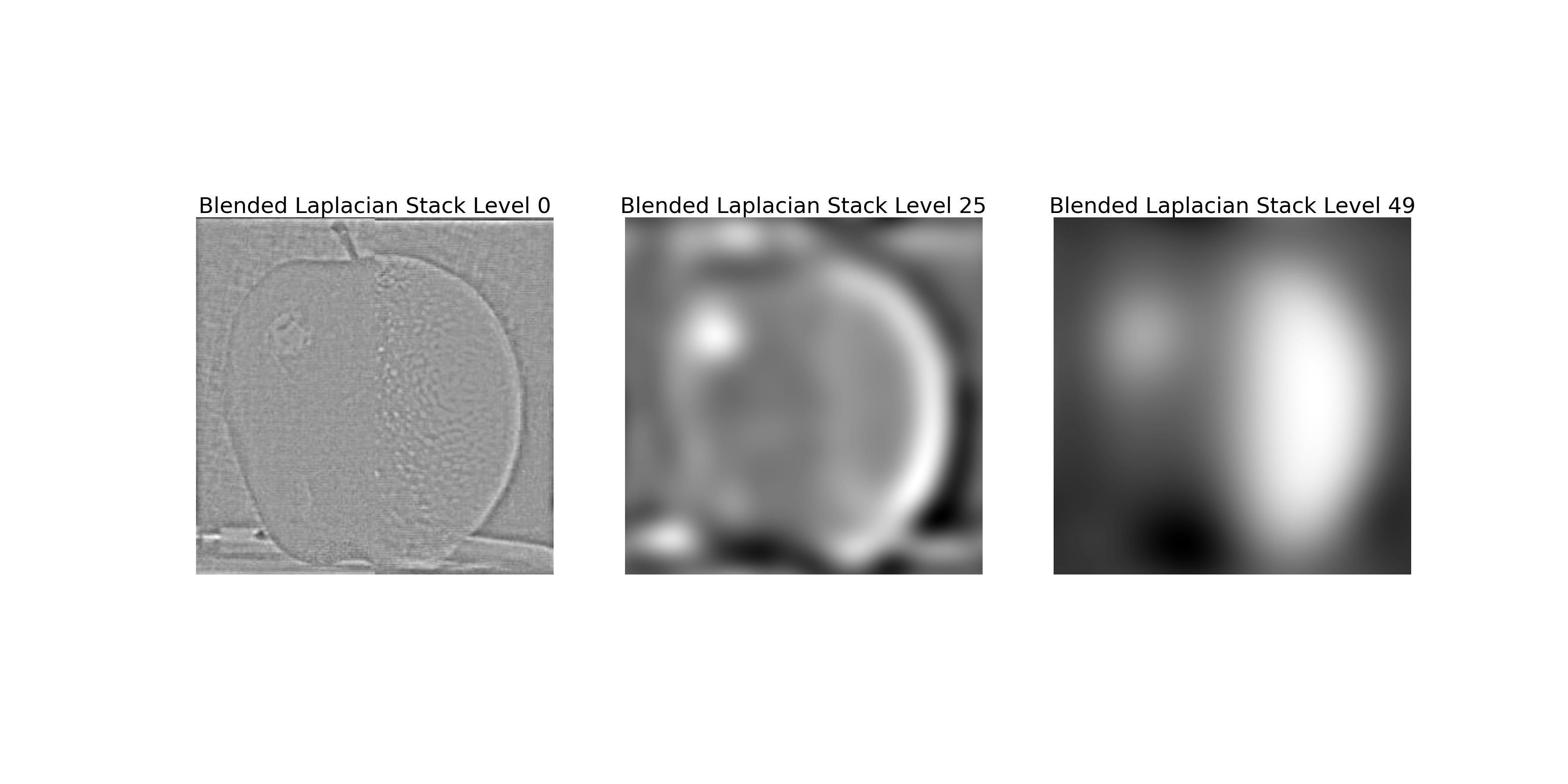
The image above shows the Laplacian stack of the blended image. This corresponds to the right column of Figure 3.42 in the textbook.
This part explores the use of multi-resolution blending to blend two images seamlessly. The blending process involves creating Gaussian and Laplacian stacks for both images, blending the corresponding levels of the Laplacian stacks, and reconstructing the blended image from the blended Laplacian stack.
We all know that minions love bananas 🍌. The following images show the blending of a banana and a minion using multi-resolution blending.

The image above shows the result of blending a banana and a minion using multi-resolution blending.
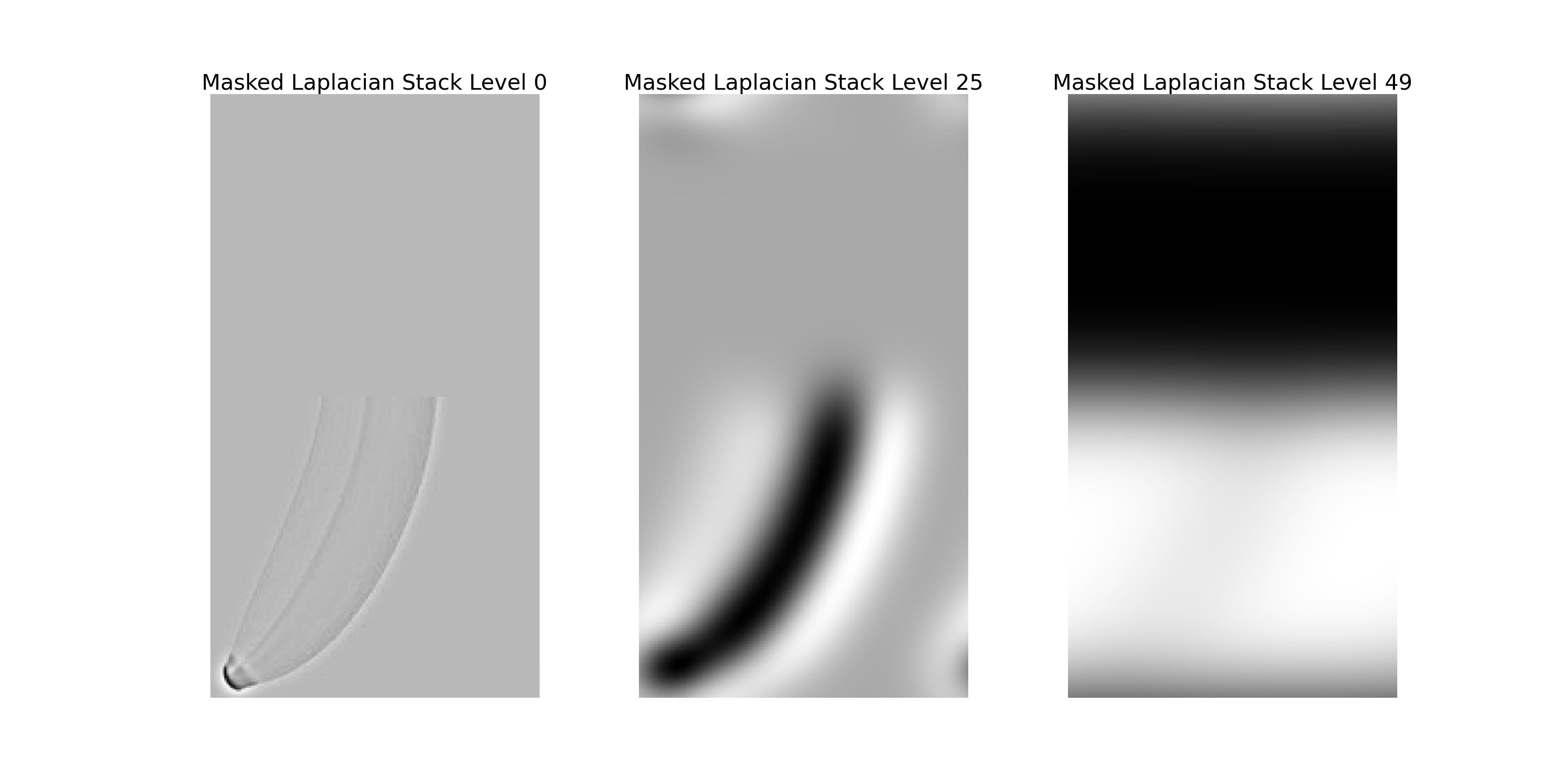
The image above shows the Laplacian stack of the banana image with the mask applied to each level.
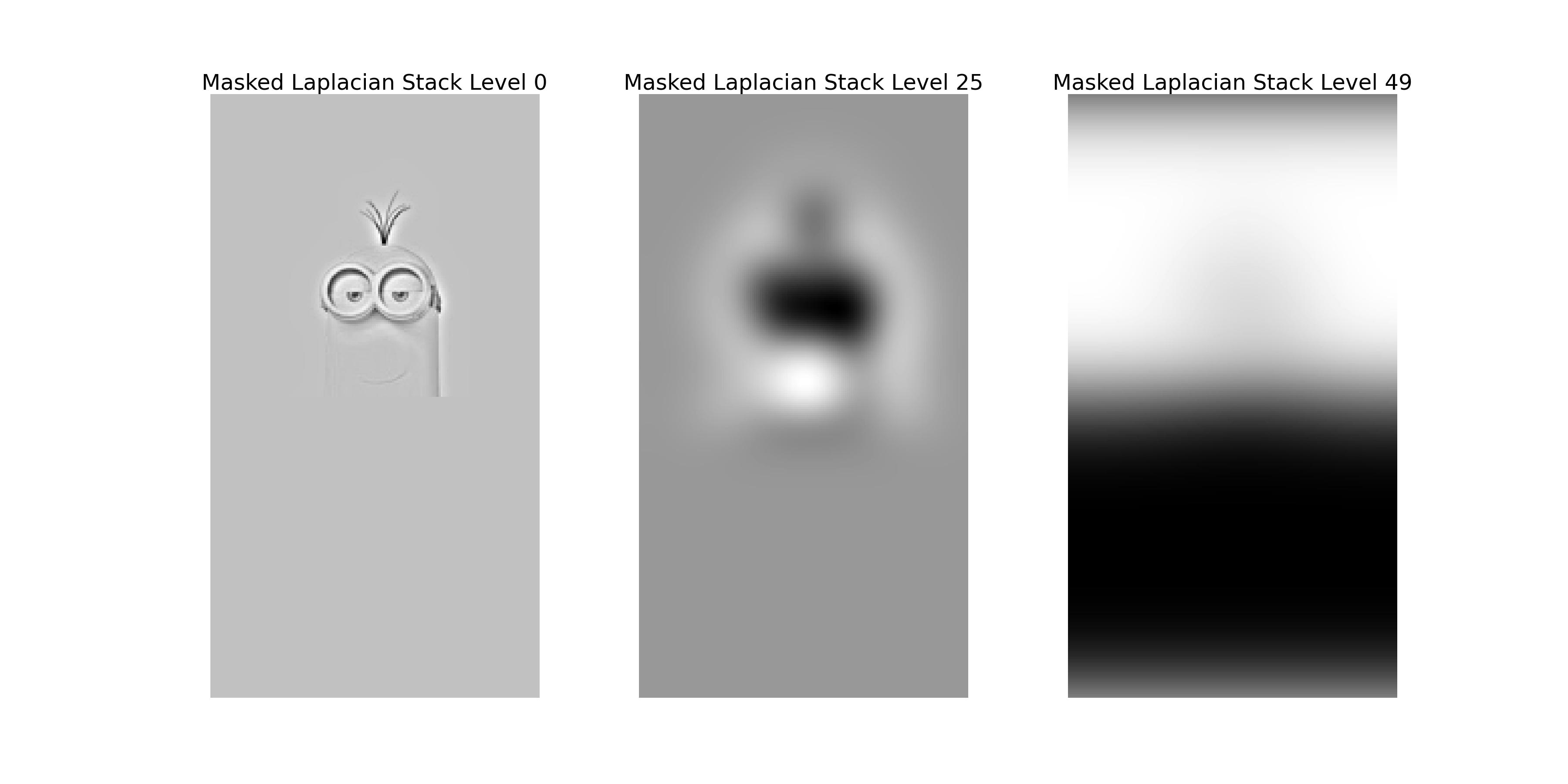
The image above shows the Laplacian stack of the minion image with the mask applied to each level.
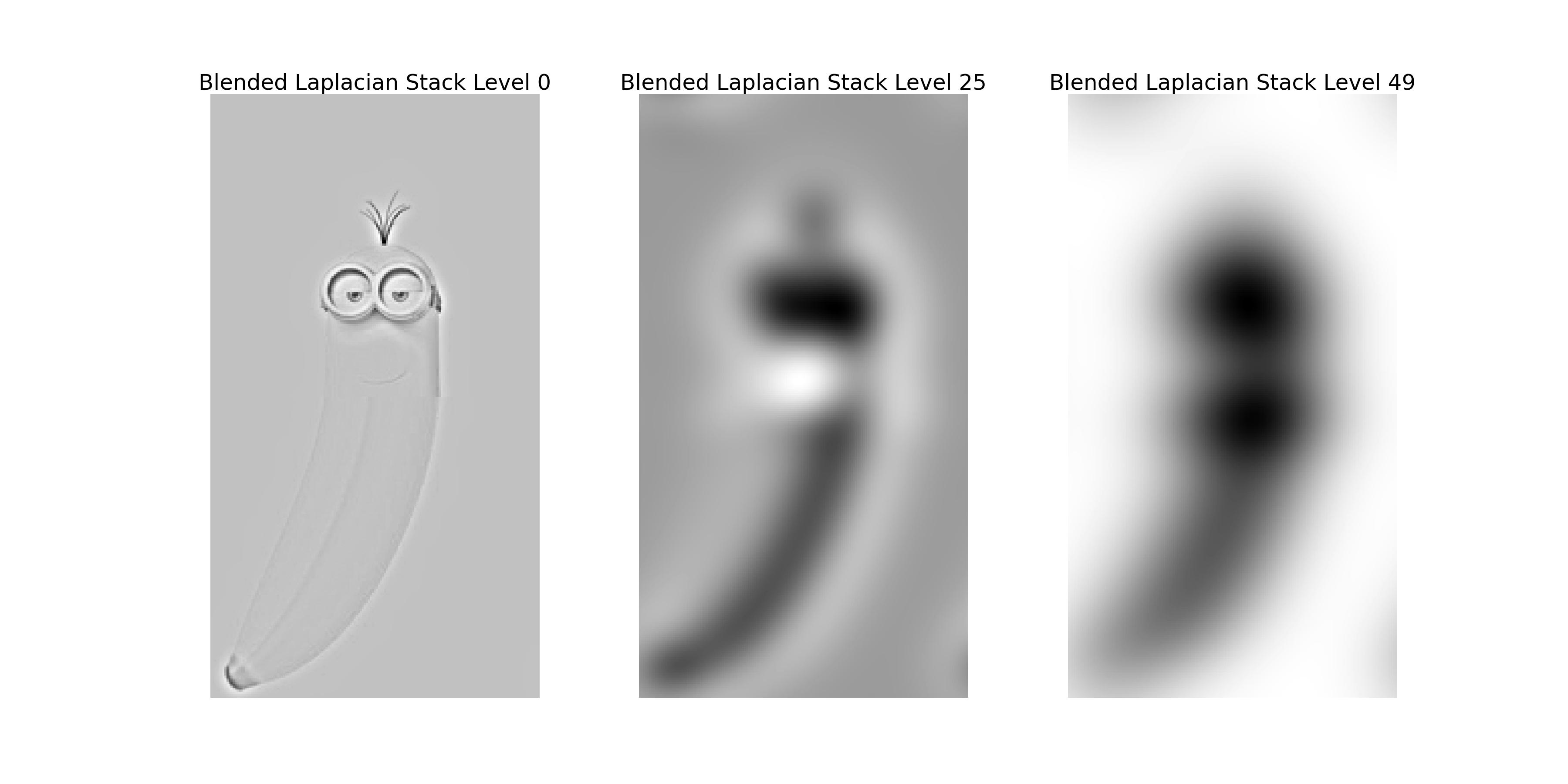
The image above shows the Laplacian stack of the blended image.
The following images show the blending of the back of a laptop and a red alarm button using multi-resolution blending.
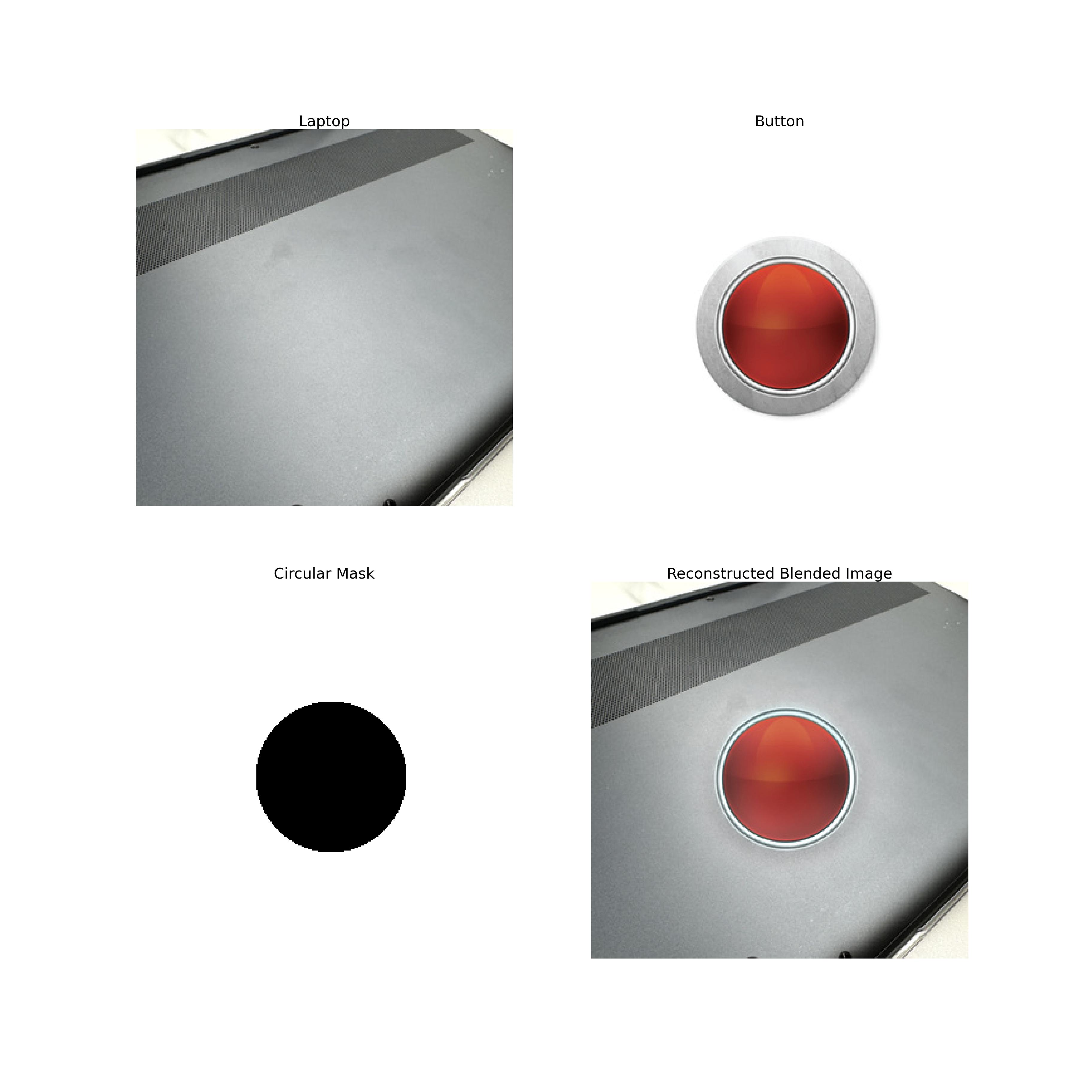
The image above shows the result of blending the back of a laptop and a red alarm button using multi-resolution blending.
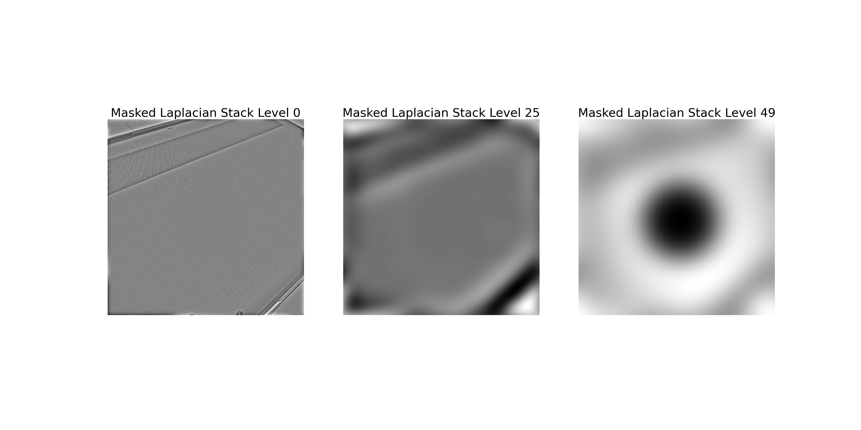
The image above shows the Laplacian stack of the laptop image with the mask applied to each level.
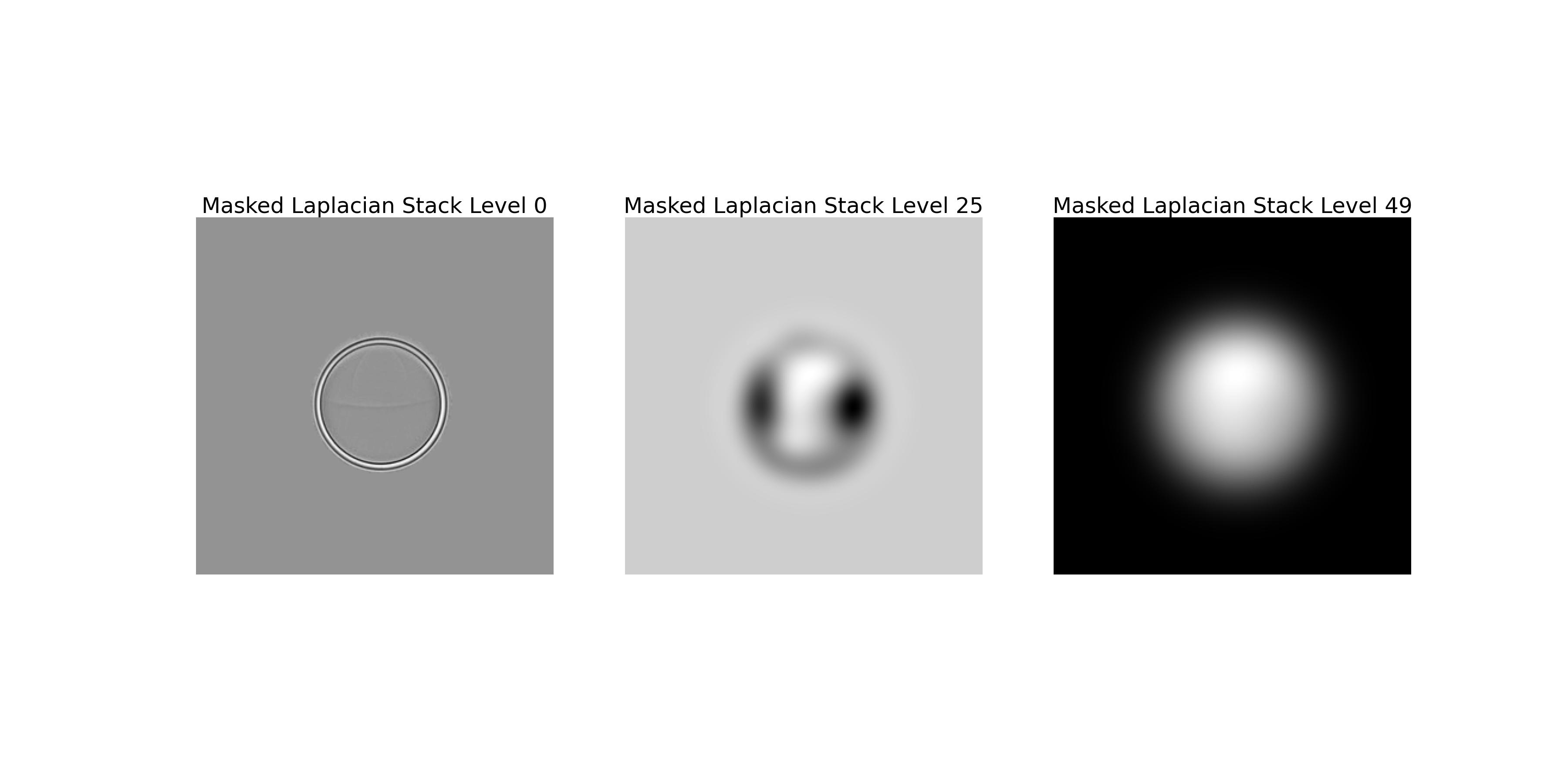
The image above shows the Laplacian stack of the button image with the mask applied to each level.
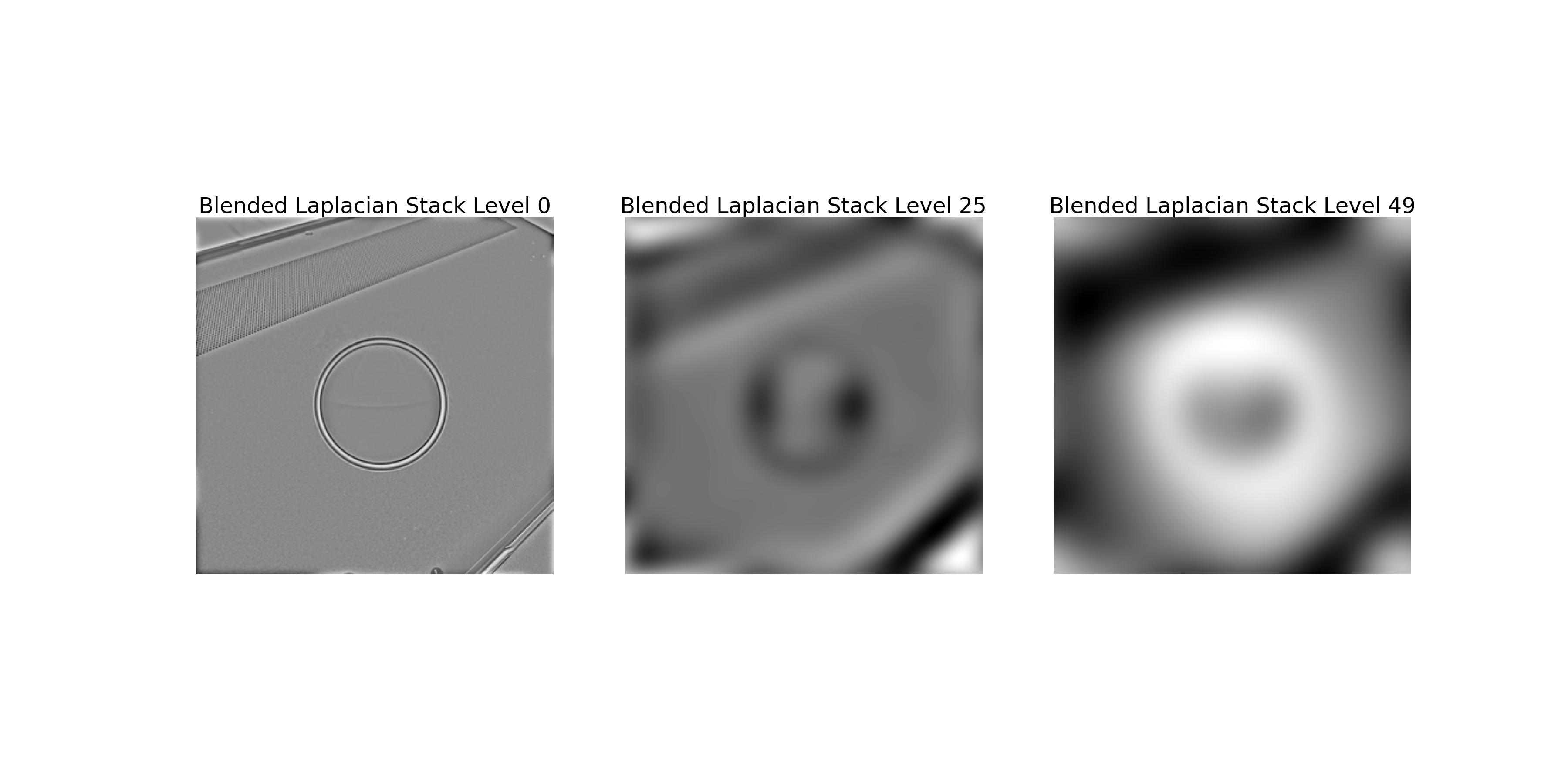
The image above shows the Laplacian stack of the blended image.