Yueheng Zeng @ Project 3
This project involves implementing face morphing and image manipulation techniques using computational photography. The primary goals are to morph an image of your face into someone else's face, compute the average face of a given population, and create a caricature by extrapolating from the population mean. Moreover, we can change the smile of an individual by adding or subtracting a "smile vector" from their face. Finally, we can perform PCA on the face shapes of the individuals in the FEI face database and generate a laughing face by altering the PCA components.


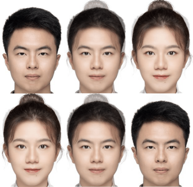
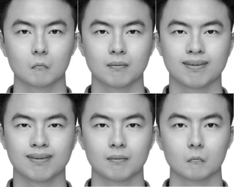
Left: Morphing from me to Ruihuan.
Right: Extrapolating from the inverse of my laughing face to
laughing face.
To define pairs of corresponding points on the two images by hand, I wrote a Python script that allows users to click on the images to select points. The script displays the images side by side and allows users to click on corresponding points on the two images. The script saves the selected points to a json file for later use.
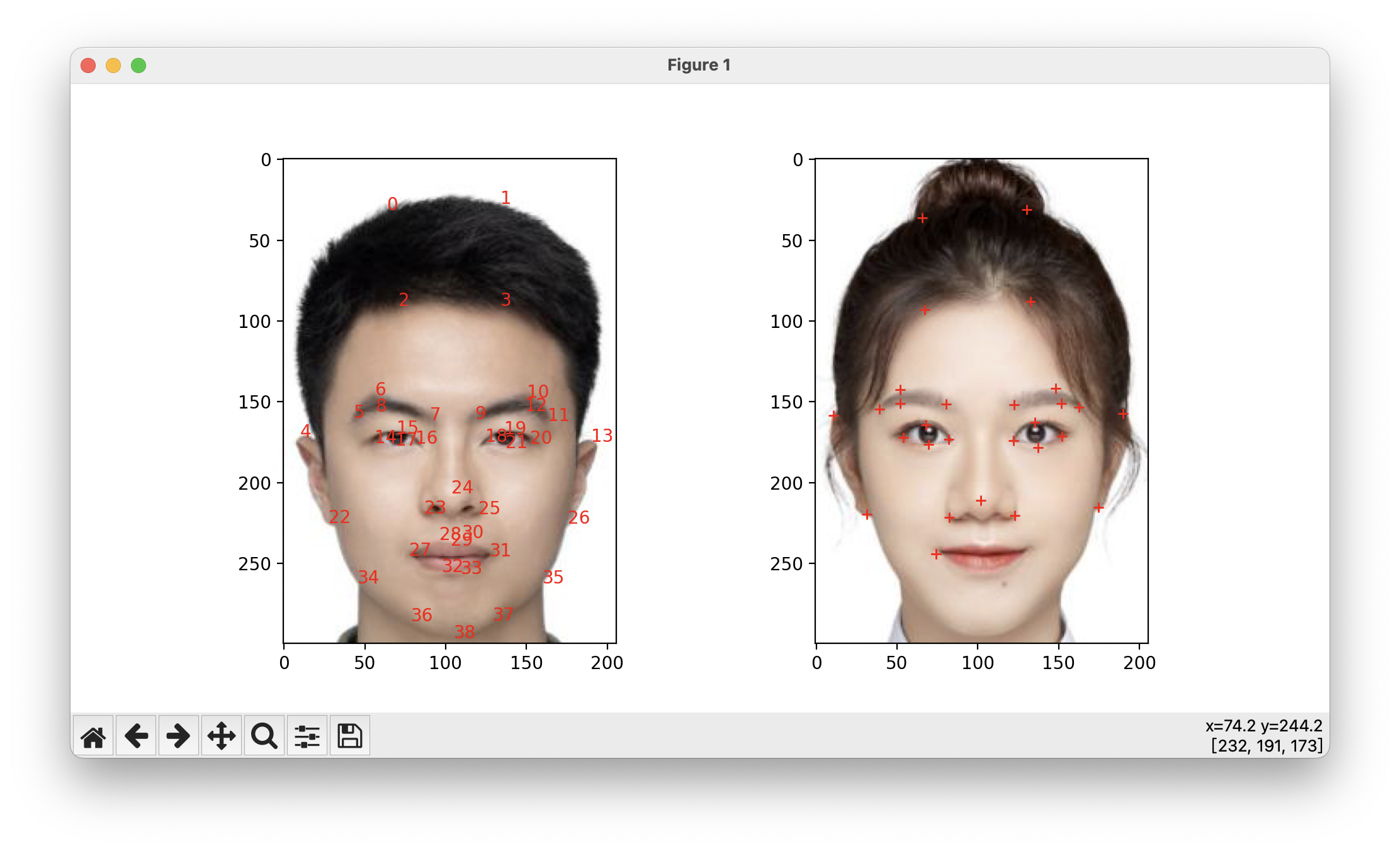
Python script for defining corresponding points on two images.
After obtaining the corresponding points, the midway shape can be computed by averaging the corresponding points. Then, the Delaunay triangulation can be computed on the midway shape.
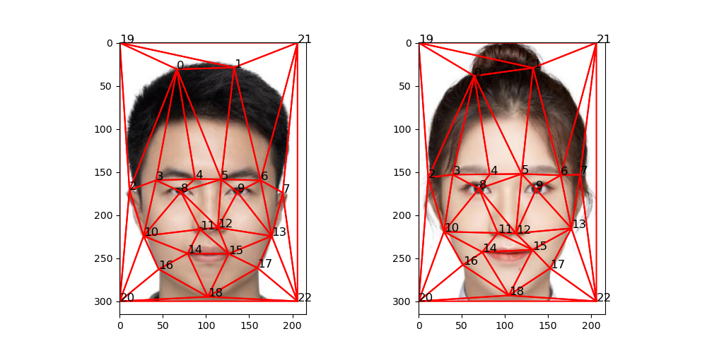
Delaunay triangulation calculated on the midway shape.
To compute the midway face, we first need to warp the two images to the midway shape already computed in the previous part. Then we average the colors of the two images to get the midway face.
To warp the images, we first compute the affine transformation matrix for each triangle in the Delaunay triangulation. The affine transformation matrix we need is defined as follows: $$ \text{target triangle} = \text{affine matrix} \times \text{source triangle} $$ where the source triangle and target triangle are defined as follows: $$ \text{source triangle} = \begin{bmatrix} x_1 & x_2 & x_3 \\ y_1 & y_2 & y_3 \\ 1 & 1 & 1 \end{bmatrix} $$ $$ \text{target triangle} = \begin{bmatrix} x'_1 & x'_2 & x'_3 \\ y'_1 & y'_2 & y'_3 \\ 1 & 1 & 1 \end{bmatrix} $$ And the affine matrix is defined as follows: $$ \text{affine matrix} = \begin{bmatrix} a & b & c \\ d & e & f \\ 0 & 0 & 1 \end{bmatrix} $$ We can see that the affine matrix has 6 unknowns, and we can solve for these unknowns by solving the linear system as follows: $$ \text{affine matrix} = \text{target triangle} \times \text{source triangle}^{-1} $$
To avoid holes in the warped image (midway face), we can use the inverse warping technique. Instead of warping the source image to the midway face, we warp the midway face to the source image. For a point \( (x_{mid}, y_{mid}) \) in the midway face, we can find the corresponding point in the source image with \( (x_{src}, y_{src}) \) by the following formula: $$ (x_{src}, y_{src}, 1) = \text{affine matrix} \times (x_{mid}, y_{mid}, 1) $$ However, the above formula may result in fractional coordinates in the source image. To solve this problem, we can use interpolation to get the pixel value at the fractional coordinates. This can be easily done using the scipy.interpolate.griddata function. Since this function is slow, we can use it after we have computed the affine matrix for all the triangles.
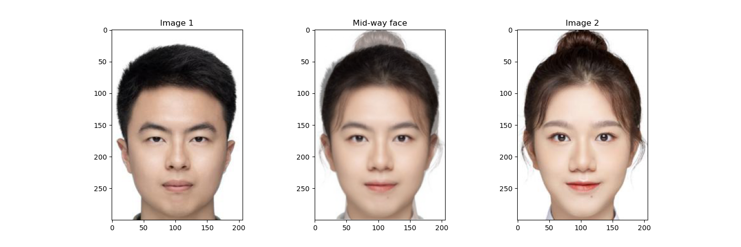
Midway face computed from me and Ruihuan.
To create the morph sequence, the only difference from the previous part is that we need involve two parameters: the parameter to control the intermidiate shape and the parameter to control the color blending. They are defined as follows: $$ \text{warp fraction} = \frac{t}{\text{number of frames} - 1} $$ $$ \text{color fraction} = \frac{t}{\text{number of frames} - 1} $$ where \( t \) ranges from \( 0 \) to \( \text{number of frames} - 1 \). By looping through all the frames, we can create the morph sequence. Moreover, if we want to create a ping-pong effect (morphing from the source to the target and then from the target), we can just append the morph sequence with the morph sequence in reverse order.

Morph sequence from me to Ruihuan.
The dataset used in this part is the FEI face database. The dataset has spatially normalized images of frontal faces of 200 individuals with 46 annonated points. Each of the individuals has an image with a neutral expression and an image with a laughing expression. Therefore, we can compute the mean face of neutral expressions and the mean face of laughing expressions.
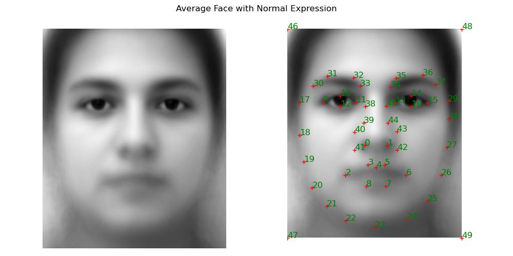
Mean face of neutral expressions.
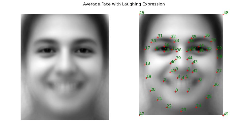
Mean face of laughing expressions.
With the mean face of laughing expressions, we can make some individuals laugh by warping their neutral expressions to the mean face of laughing expressions. Some of the results are shown below.
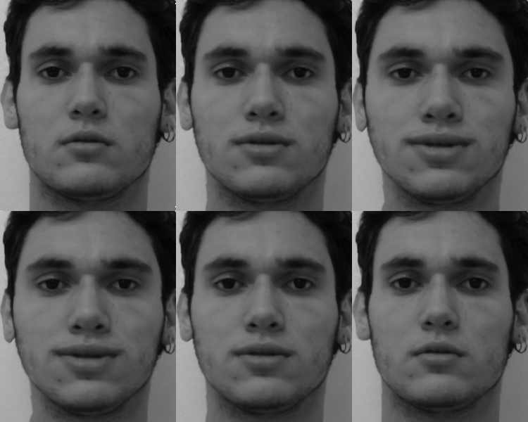
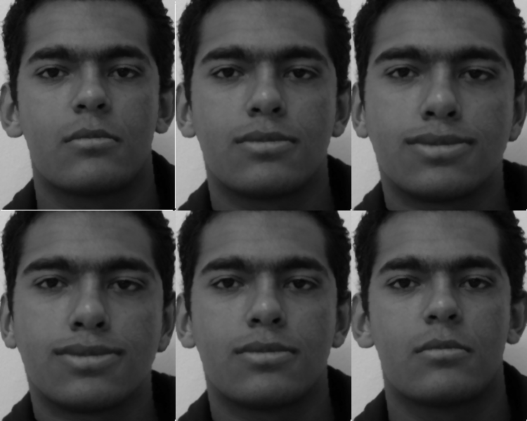

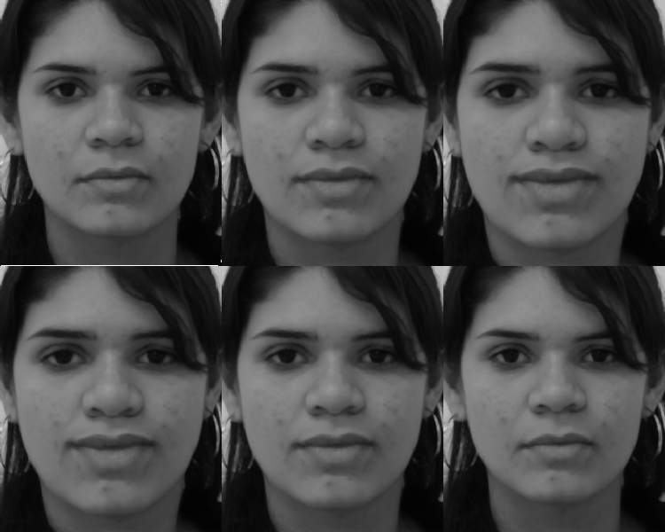
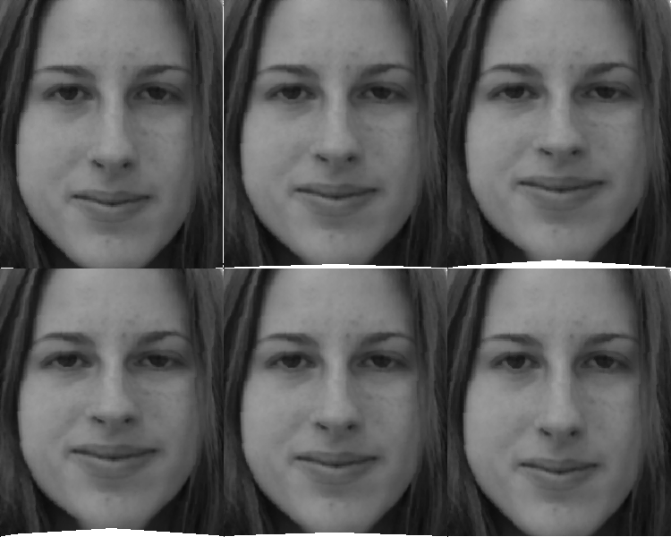
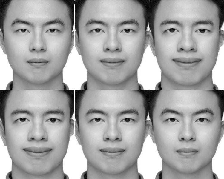
The first five images are individuals from the FEI face database. The last image is me.
We can see that the results better on those individuals in the FEI face database than on me. This might be because the individuals in the FEI face database have a more similar face shape to the mean face of laughing expressions than me.
To create a caricature of my face, we can extrapolate from the mean face of Chinese males to my face. The process can be shown as follows: $$ \text{extrapolate vector} = \text{my face shape} - \text{mean face shape} $$ $$ \text{caricature shape} = \text{mean face shape} + \text{factor} \times \text{extrapolate vector} $$ where the factor is a parameter to control the exaggeration of the caricature.
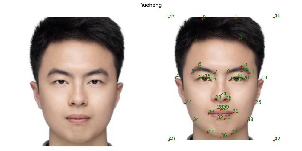
My face.
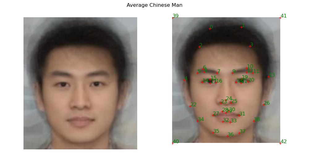
Mean face of Chinese males.
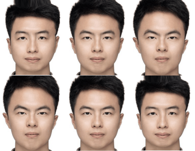
Caricature of my face from the mean face with factor -1 to 1.
To change the smile of an individual, we can subtract the mean face of neutral expressions from the mean face of laughing expressions to get the smile vector. Then we can add the smile vector to the individual's face to make them smile.

Smile vector applied to my face.
If we subtract the smile vector from someone's face, we can make them not smile, or even make them frown.
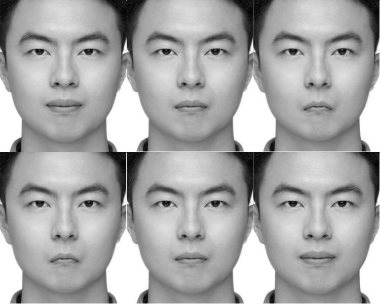
Inverse smile vector applied to my face.
To perform PCA on the face shapes of the individuals in the FEI face database, we first need to flatten the face shapes into vectors (one vector for each face shape, each has 100 dimensions). Then we need to standardize the vectors. After that, we can perform PCA on the standardized vectors.
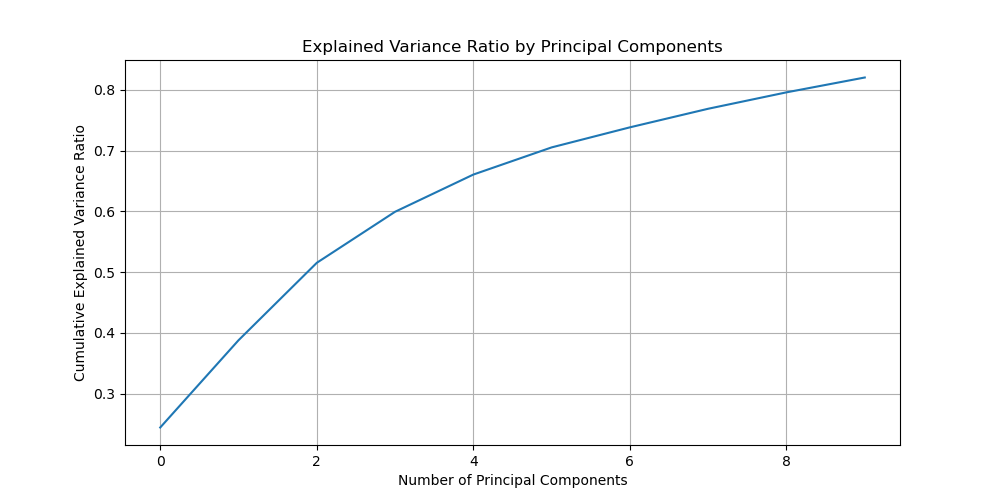
Explained variance ratio of the PCA.
We can see that just the first 10 PCA components can explain 80% of the variance in the data. Therefore, it is reasonable to use the first 10 PCA components as the basis for the face shapes.
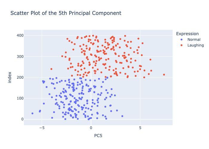
Scatter plot of the fifth PCA component.
We can see that the fifth PCA component is positively correlated with the smile of the face shapes. We can further confirm this by projecting the smile vector to the PCA basis and see that the smile vector is mostly aligned with the fifth PCA component.
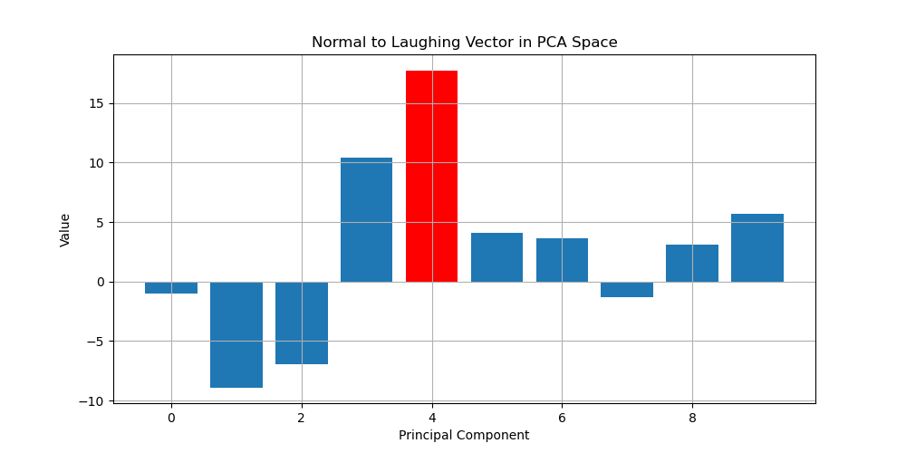
Smile vector projected to the PCA basis.
We can see that the smile vector has high values on the fifth PCA component. Therefore, we can generate a laughing face by increasing the fifth PCA component or adding the smile vector to the face. The results are shown below.

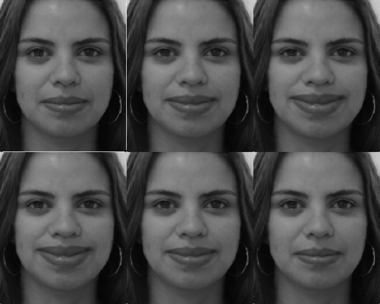
Left: Laughing face generated by increasing the fifth PCA component.
Right: Laughing face generated by adding the smile vector to the face.
We can see that the result on the left is similar to the result on the right. So in this case, making transformations in the PCA space similar to making transformations in the normal basis.