Yueheng Zeng @ Project 4
This project focuses on auto stitching photo mosaics. It is divided into two main parts: the first involves capturing source images, establishing correspondences, and manually warping and compositing them into a mosaic. The second part aims to automate the correspondence-finding process from Part 1, allowing for the efficient creation of these composite images.

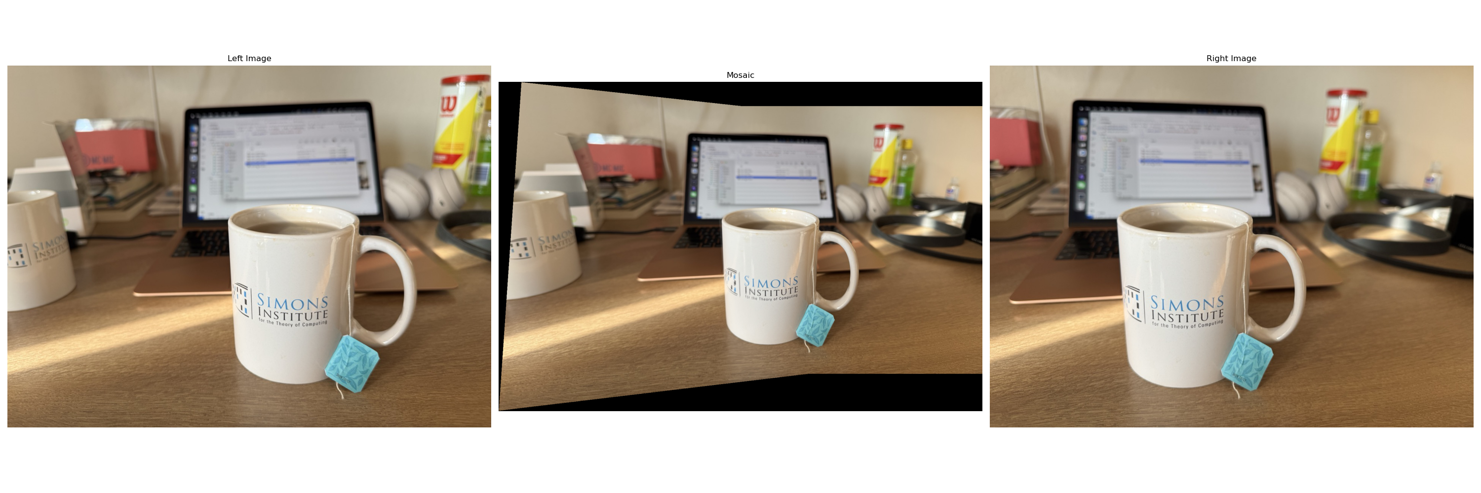
Automatically stitched mosaic of my deck.
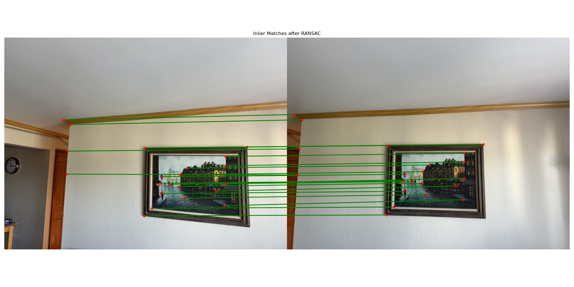
Automatically detected inlier matches between the two images in my living room.
To be able to create a mosaic of two images, we first need to take two pictures of the same scene from different angles but with the same center of projection. The two images should have a significant overlap between them. I took two pictures of my living room from two different angles with my phone camera.
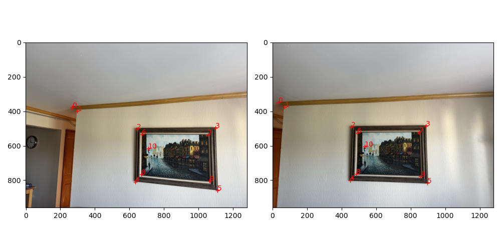
My two images of the living room with defined correspondences.
The homography matrix \(\mathbf{H}\) describes a transformation between two planes. Given a set of corresponding points from two images, we aim to compute the homography matrix that maps points from one image to the other. Let the correspondence between the two images be given by points \(\mathbf{p}_1 = (x_1, y_1)\) in the first image and \(\mathbf{p}_2 = (x_2, y_2)\) in the second image. The homography relates these points via the equation: \[ \begin{bmatrix} x_2 \\ y_2 \\ 1 \end{bmatrix} \propto \mathbf{H} \begin{bmatrix} x_1 \\ y_1 \\ 1 \end{bmatrix}. \] The goal is to compute the \(3 \times 3\) homography matrix \(\mathbf{H}\) For each pair of corresponding points \(\mathbf{p}_1 = (x_1, y_1)\) and \(\mathbf{p}_2 = (x_2, y_2)\) we derive two linear equations from the homography relationship: \[ \begin{aligned} x_2 &= h_{11} x_1 + h_{12} y_1 + h_{13} - h_{31} x_1 x_2 - h_{32} y_1 x_2, \\ y_2 &= h_{21} x_1 + h_{22} y_1 + h_{23} - h_{31} x_1 y_2 - h_{32} y_1 y_2. \end{aligned} \] Rearranging these into a system of equations for \(n\) pairs of points leads to the matrix form: \[ \mathbf{A} \mathbf{h} = \mathbf{b}, \] where \(\mathbf{A}\) is a \(2n \times 8\) matrix constructed from the points in the first image, and \(\mathbf{b}\) is a \(2n \times 1\) vector constructed from the points in the second image. For each correspondence, the rows of \(\mathbf{A}\) are given by: \[ \mathbf{A} = \begin{bmatrix} x_1 & y_1 & 1 & 0 & 0 & 0 & -x_1 x_2 & -y_1 x_2 \\ 0 & 0 & 0 & x_1 & y_1 & 1 & -x_1 y_2 & -y_1 y_2 \end{bmatrix}, \] and the vector \(\mathbf{b}\) is: \[ \mathbf{b} = \begin{bmatrix} x_2 \\ y_2 \end{bmatrix}. \] To compute the homography matrix, we solve the least-squares problem: \[ \mathbf{h} = \text{argmin} \|\mathbf{A} \mathbf{h} - \mathbf{b}\|. \] This is solved using the function np.linalg.lstsq, which provides the best-fit solution to this system. The resulting vector \(\mathbf{h}\) contains the first 8 elements of the homography matrix. The final element \(h_{33}\) is set to 1, and \(\mathbf{h}\) is reshaped into a \(3 \times 3\) matrix: \[ \mathbf{H} = \begin{bmatrix} h_{11} & h_{12} & h_{13} \\ h_{21} & h_{22} & h_{23} \\ h_{31} & h_{32} & 1 \end{bmatrix}. \]
To warp an image, we need to apply the homography matrix \(\mathbf{H}\) to each pixel in the image. To determine the size of the destination image, we first apply the homography to the four corners of the source image. The destination image is then defined as the bounding box that contains all the transformed corner points. If the warped corner points are negative, we shift the image to ensure all points are positive.
To avoid holes in the destination image, we can adopt the inverse warping approach. For each pixel \((x, y)\) in in the destination image, we compute the corresponding pixel \((x', y')\) in the source image by applying the inverse homography matrix \(\mathbf{H}^{-1}\): \[ \begin{bmatrix} x' \\ y' \\ 1 \end{bmatrix} \propto \mathbf{H}^{-1} \begin{bmatrix} x \\ y \\ 1 \end{bmatrix}. \] The pixel \((x', y')\) is then interpolated from the source image to the destination image using bilinear interpolation.
After implementing the warp function, we can rectify elements in the image. To rectify an element, we need to compute the homography matrix that maps the element to a rectangle. We can then apply the warp function to the element to rectify it.
In the example below, I rectified the picture frame in my living room by letting the four corners of the frame map to the four corners of a rectangle. The resulting rectified frame is shown below.
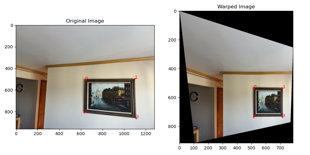
Rectified picture frame in my living room.
To blend the images into a mosaic, we can project one image onto the other using the homography matrix. In the example below, I warped the first image onto the second image, and created a mask with the warped pixels in the first image being set to 1 and the rest to 0. From the result, we can see that the key points are well aligned, and the two images are ready to be blended.
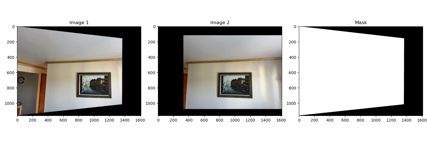
Warped image 1, Expanded image 2, and Mask.
To blend the images, we can directly blend the images using the mask we just created. The blending is done by setting the pixel value to the first image if the mask is 1 and the second image if the mask is 0. The result is shown below. We can see that the two images are well blended into a mosaic. However, the blending is not perfect, and we can see a boundary between the two images.

Direct blending of the two images.
To improve the blending, we can cross dissolve the images at the overlapping region. The cross-dissolve can be done with the following masks that linearly interpolate between the two images.
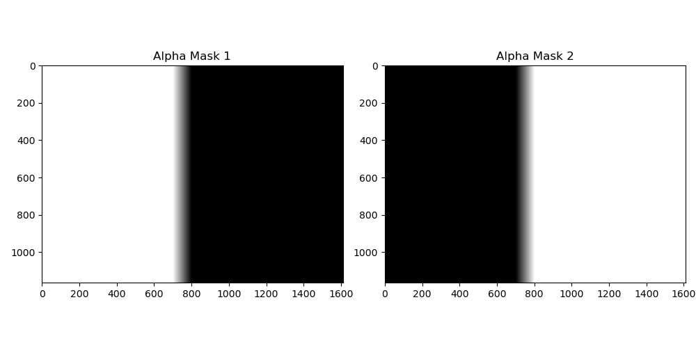
Alpha masks for cross-dissolve.
We can then blend the images using the masks above. As for those pixels that are not in the overlapping region, we can directly blend the images using the mask we created earlier. The result is shown below. We can see that the blending is much smoother, and the boundary between the two images is not visible.
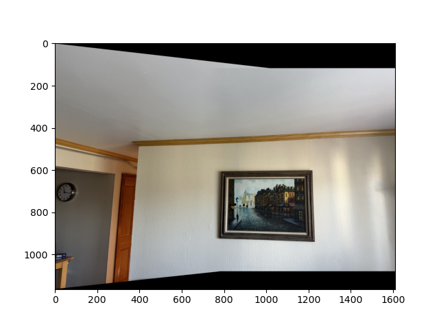
Cross-dissolve blending of the two images.
To detect corner features in an image, we can use the Harris corner detector. The Harris corner detector computes the corner response function \(R\) for each pixel in the image. The response function is given by: \[ R = \text{det}(\mathbf{M}) - k \cdot \text{trace}(\mathbf{M})^2, \] where \(\mathbf{M}\) is the structure tensor of the image, and \(k\) is a constant. The structure tensor is defined as: \[ \mathbf{M} = \begin{bmatrix} I_x^2 & I_x I_y \\ I_x I_y & I_y^2 \end{bmatrix}, \] where \(I_x\) and \(I_y\) are the image gradients in the \(x\) and \(y\) directions, respectively. The Harris corner detector computes the corner response function for each pixel in the image. The pixels with high corner response values are considered corners. By calling the function skimage.feature.corner_harris and skimage.feature.peak_local_max, we can detect the corner features in the image.

Detected corner features in the left image.
The Adaptive Non-Maximal Suppression algorithm selects a subset of interest points from detected corners in an image based on their strength, aiming to preserve the most significant features while reducing redundancy. The algorithm begins by extracting and sorting corner strengths, then computes suppression radii for each corner based on the distance to stronger corners while considering their strength relative to a specified threshold. Finally, it selects the top features based on these radii, returning the coordinates of the most significant corners that maximize both strength and spatial distribution.
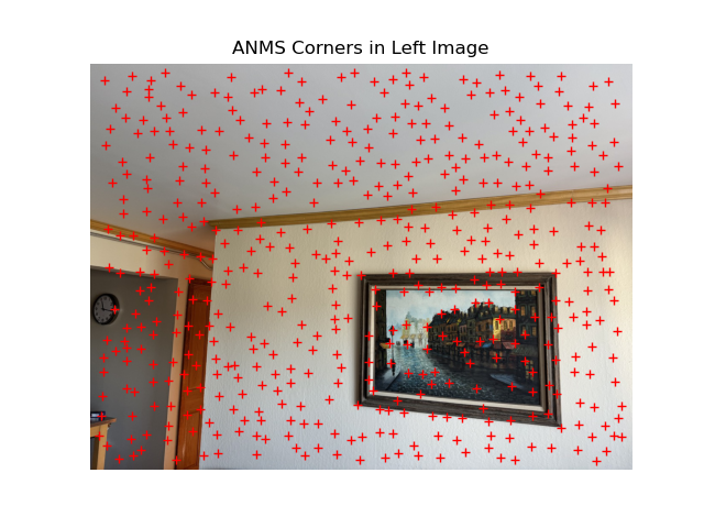
Selected corners in the left image using adaptive non-maximal suppression.
Feature descriptors are created by initially extracting pixel values from a 40x40 window centered on the detected corners. These pixel values are then downsampled to an 8x8 patch and normalized to achieve zero mean and unit variance. Finally, the normalized values are reshaped into a 64-dimensional vector, representing the corner's feature descriptor.
Feature matching is performed by using the Lowe's ratio test. For a descriptor in the first image, we find the two closest descriptors in the second image based on Euclidean distance. If the ratio of the nearest to the second-nearest distance is below a specified threshold, the pair is considered a match. This process is repeated for all descriptors in the first image, resulting in a set of matched feature pairs.
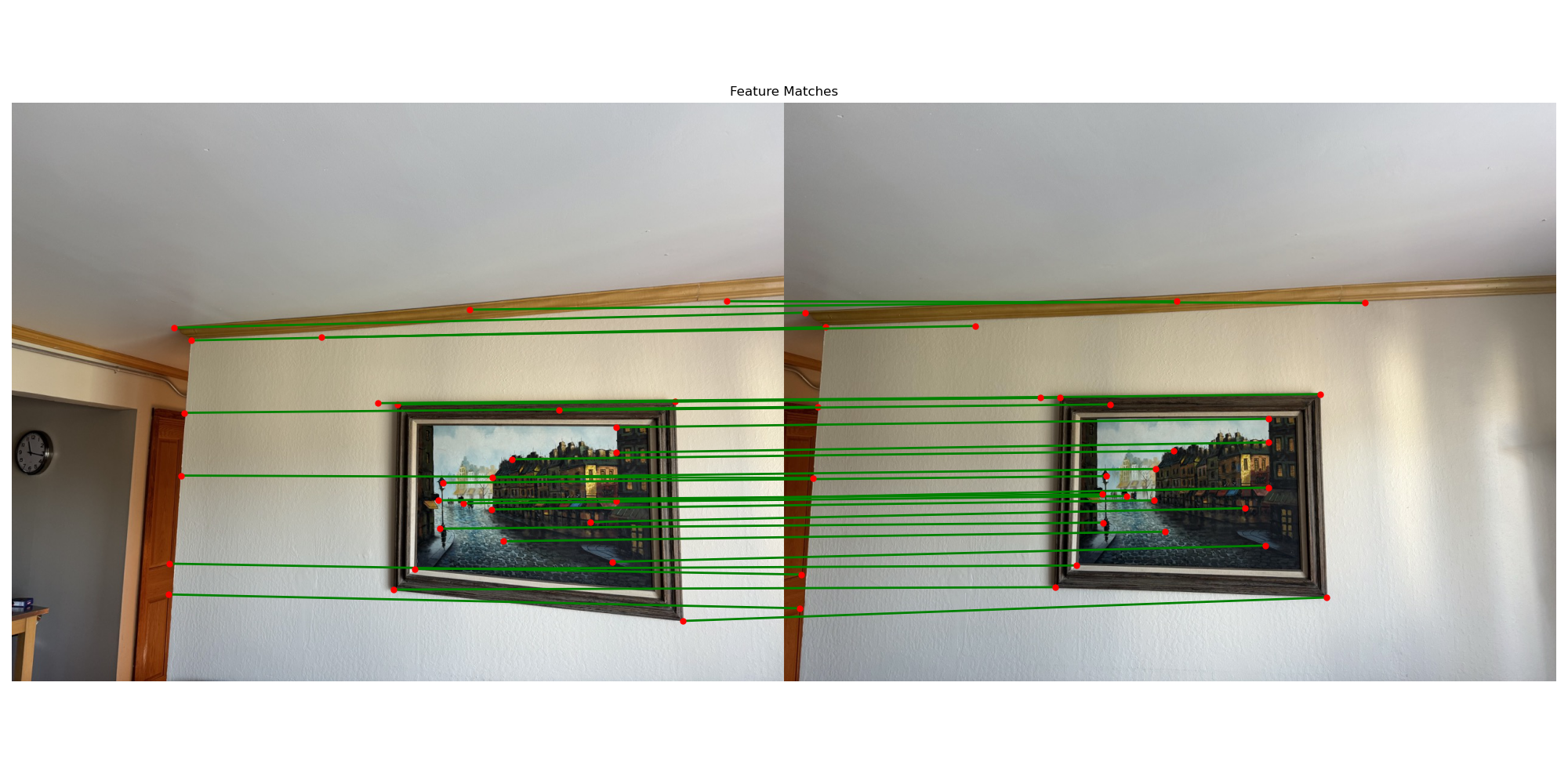
Matched features between the two images.
The RANSAC algorithm is used to select a robust set of feature matches to compute a homography matrix. The algorithm iteratively selects a random subset (in our case, 4 pairs) of feature matches to compute a homography matrix. The homography matrix is then used to warp the matched points from the first image to the second image. The number of inliers is computed by comparing the warped points to the actual points in the second image. The subset of feature matches with the most inliers is considered the best set of matches, and the homography matrix is re-computed using all the inliers.

Inlier matches between the two images.
With the homography matrix computed from RANSAC, we can now automatically stitch the two images together. The first image is warped onto the second image using the homography matrix. The two images are then blended together using the alpha blending technique described in Part 4A.
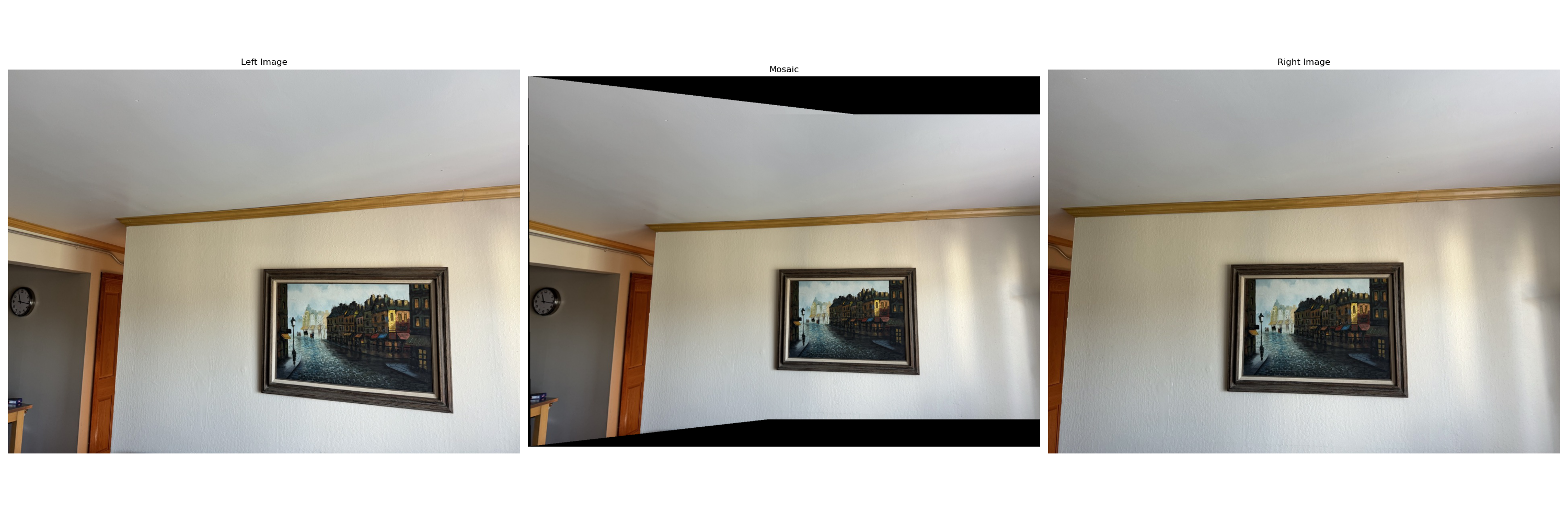
Automatically stitched mosaic of my living room.

Manually stitched mosaic of my living room.
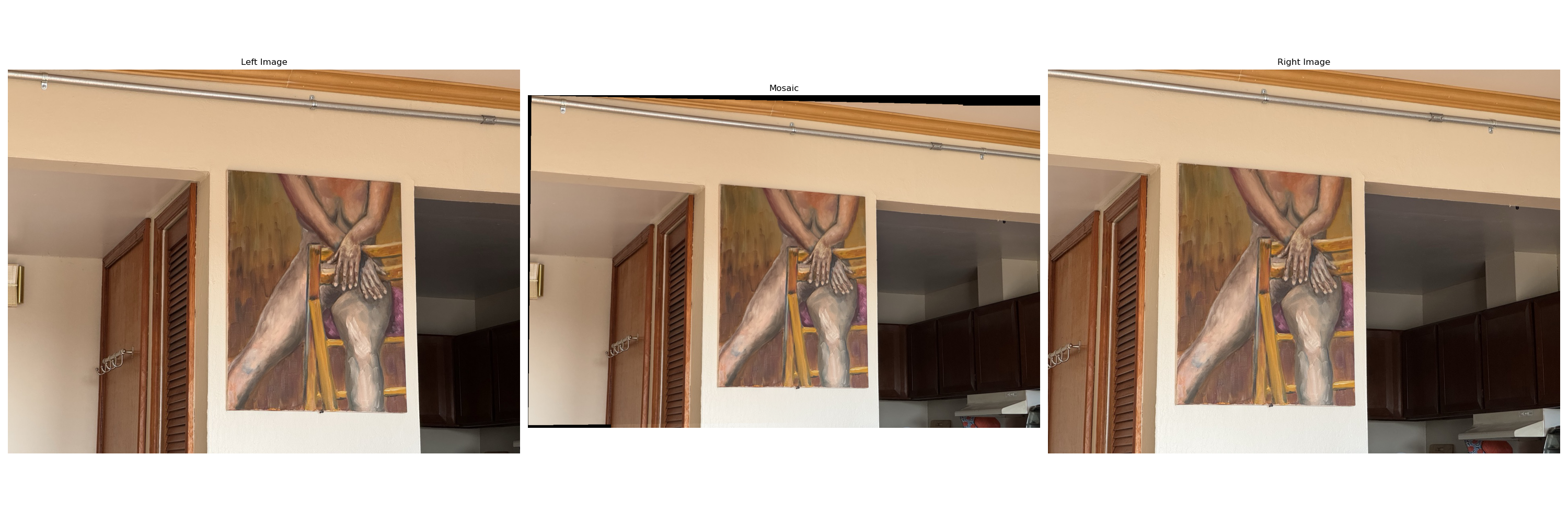
Automatically stitched mosaic of my living room.

Automatically stitched mosaic of my deck.
The most exciting thing I learned from this project was how to automatically stitch two images together. I discovered how to detect corner features in an image, extract feature descriptors, and match features between two images. Additionally, I learned to compute a robust homography matrix using RANSAC.
Among all the techniques I explored, I found feature extraction to be the most intriguing. It's fascinating to see how efficiently we can extract features from a point in an image by analyzing its surrounding pixels. These surrounding pixels can be easily organized into a vector through downsampling and normalization, and this straightforward method yields surprisingly effective results!